COVID-19 Pandemic and Financial Contagion - MDPI
←
→
Page content transcription
If your browser does not render page correctly, please read the page content below
Journal of
           Risk and Financial
           Management

Article
COVID-19 Pandemic and Financial Contagion
Julien Chevallier 1,2
 1    Department of Economics & Management, IPAG Business School (IPAG Lab), 184 bd Saint-Germain,
      75006 Paris, France; julien.chevallier@ipag.fr
 2    Economics Department, Université Paris 8 (LED), 2 rue de la Liberté, CEDEX 93526 Saint-Denis, France

 Received: 15 October 2020; Accepted: 1 December 2020; Published: 3 December 2020

 Abstract: The original contribution of this paper is to empirically document the contagion of the
 COVID-19 on financial markets. We merge databases from Johns Hopkins Coronavirus Center,
 Oxford-Man Institute Realized Library, NYU Volatility Lab, an d St-Louis Federal Reserve Board.
 We deploy three types of models throughout our experiments: (i) the Susceptible-Infective-Removed
 (SIR) that predicts the infections’ peak on 2020-03-27; (ii) volatility (GARCH), correlation (DCC),
 and risk-management (Value-at-Risk (VaR)) models that relate how bears painted Wall Street red;
 and, (iii) data-science trees algorithms with forward prunning, mosaic plots, and Pythagorean forests
 that crunch the data on confirmed, deaths, and recovered COVID-19 cases and then tie them to
 high-frequency data for 31 stock markets.

 Keywords: COVID-19; financial contagion; Johns Hopkins repository; Susceptible-Infective-Removed
 model; tree algorithm; data science

1. Introduction
      The COVID-19 pandemic hit the world economy, without anyone knowing, at light-speed, leading
to partial unemployment and factories’ shutdown around the globe, leaving doctors, policymakers,
businessmen, operational managers, data scientists, and citizens alike in disarray. The origin of the
virus itself is not known with certainty, although most theories attach it to zoonotic transfer to the
human species (Andersen et al. 2020).
      As such, the COVID-19 virus outbreak represents a pandora’s box. The original 45-day lock-down
in most industrialized countries dated mid-March 2020 took everybody off-guard. This paper aims to
address many viewpoints (e.g., business cycle analysis, operational research impediments, open-data
science) during this traumatizing event.
      With the quarantine in action in most industrialized countries from mid-March until the
end-of-year 2020, many economist observers predict a deep recession for 2021–22. Stock markets
plunged in March–April 2020, due to the shocking news of the virus spreading around the world.
      Literature on the financial impacts of the COVID-19 is burgeoning. Akhtaruzzaman et al. (2020)
examine how financial contagion occurs through financial and nonfinancial firms between China and
G7 countries during the COVID–19 period. Ashraf (2020) finds that stock market returns declined as
the number of COVID-19 confirmed cases increased. Among the main driving forces, government
restrictions on commercial activity and voluntary social distancing are the main reasons behind the U.S.
stock market plunge (Baker et al. 2020). On the Chinese stock market, Al-Awadhi et al. (2020) confirm
that the daily growth in the total confirmed cases and total cases of death caused by COVID-19 both
have significant negative effects on stock returns across all companies. Papadamou et al. (2020) suggest
that Google-based anxiety regarding COVID-19 contagion effects leads to elevated risk-aversion in
stock markets. Sharif et al. (2020b) analyze the connectedness between the recent spread of COVID-19,
oil price volatility shock, the stock market, geopolitical risk, and economic policy uncertainty in

J. Risk Financial Manag. 2020, 13, 309; doi:10.3390/jrfm13120309                   www.mdpi.com/journal/jrfm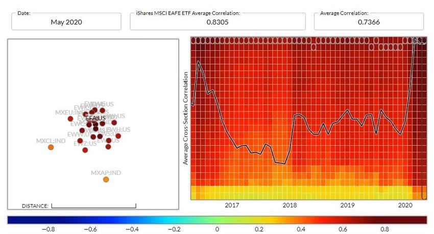
J. Risk Financial Manag. 2020, 13, 309                                                                                    2 of 25

the US within a time-frequency framework. Regarding the stringency of policy responses to the
novel coronavirus pandemic worldwide, Zaremba et al. (2020) demonstrate that non-pharmaceutical
interventions significantly increase equity market volatility. Ji et al. (2020) evaluate the safe-haven role
of assets in the current COVID-19 pandemic (gold and soybean futures). Shifting away from traditional
asset markets, Conlon and McGee (2020) show that a small allocation to Bitcoin substantially increases
portfolio downside risk: cryptocurrencies move in lockstep with the S&P 500 as the crisis develops.
In the same vein, Cheema et al. (2020) identify that, during COVID, investors might have lost trust
in gold. The US dollar has acted as a safe haven only for China and India during COVID. However,
tether can be seen as a strong safe-haven.
      In this paper, we seek to analyze how the sanitary crisis impacted economic activity based on
various methodological frameworks: a Susceptible-Infective-Removed model (epidemiology); GARCH,
Dynamic Conditional Correlation, and Value-at-Risk (finance); Decision Tree Algorithm with Forward
Pruning, Mosaic Plot, and Pythagorean Forest (data science).
      The study unfolds by (i) reporting statistics and evidence on the evolution of the pandemic,
(ii) analyzing the impact of the crisis on financial markets, and (iii) presenting a case study regarding
how data science can be applied to link financial data to Covid-data.
      From a financial contagion1 viewpoint, we uncover a wealth of insights that are related to the
COVID-19 virus outbreak. According to the infectious model, the most noticeable result was the
world’s infection “peak” detected on 3 March. According to the decision tree, the virus contamination
has been irrigating worldwide stock markets since mid-March 2020, stemming from Western Europe’s
France CAC 40 (with President Macron establishing 45-day lock-down on 16 March).
      The article’s motivation is to elaborate, against the pandemic background, a data-driven academic
assessment of the financial meltdown at stake. The article’s primary purpose is to confront many
viewpoints on the COVID-19 epidemic: medical professionals, financial analysts, and data scientists.
The goals are to retrieve scientific data in order to make statements regarding financial market
contagion. The novelty is in conducting empirical experiments from the technical standpoints of
data-science and operations research. The contribution is to be found in the financial literature by
providing several stylized facts on how financial markets react and can be expected to recover from
the COVID-19 pandemic.
      In terms of methodology, we show, using operational research models, that asset markets were
linked to the spread of the COVID-19 stocks panic across the globe. The central result is that COVID-19
triggered an unexpected panic on stock markets, which all went into losses territory. Asset managers
do not have sufficient “safe-assets” to hedge against this market panic. Therefore, the stock markets’
critical message is to wait for the COVID-19 vaccine to loom on the horizon: as more patients recover
from the disease, a new era of market gains will begin. The empirical observation that asset markets
could be re-born as patients heal and the hopes of a vaccine against COVID-19 become realistic is
genuinely novel.

1   To elaborate on the notion of “contagion” in financial econometrics, usually, the definition by Forbes and Rigobon (2002) is
    retained as a significant increase in cross-market linkages after a shock to one country (or group of countries). According to
    this definition, if two markets show a high degree of co-movement during periods of stability, even if the markets continue
    to be positively correlated after a shock to one market, then this may not constitute contagion. According to Forbes and
    Rigobon (2002)’s definition, it is only contagion if cross-market co-movement significantly increases after the shock. If the
    co-movement does not increase significantly, then any continued high level of market correlation suggests strong linkages
    between the two economies that exist in all states of the world. The term interdependence is used to refer to this situation.
    In our setting, we merely employ financial econometrics techniques (e.g., GARCH, Dynamic Conditional Correlation (DCC),
    Value-at-Risk (VaR)) in order to describe the state of disarray on financial markets given the whole pandemic situation.
    We are not interested in measuring excess co-movements. The paper’s original contribution lies in the data-scientist
    approach, instead mobilizing operational research techniques.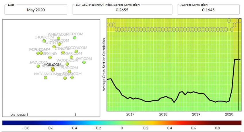
J. Risk Financial Manag. 2020, 13, 309                                                                                  3 of 25

     To retrieve data, we connected remotely to the servers of the John Hopkins Coronavirus Resource
Center2 , the Oxford-Man Institute Realized Library3 , the Volatility Lab at New York University4 , and
the St-Louis Federal Reserve Board5,6 . The time frame for the window of observations differs whether
we access only recent (newest) data, such as COVID-19 cases, or whether we download the full history
of data of prices for financial markets in order to document the current historical peaks.7
     The remainder of the article is structured, as follows. Section 2 details the latest medical evidence
on the virus. Section 3 depicts the disarray of investors. Section 4 connects the epidemiological cases
on COVID-19 to the contagion that was witnessed on financial markets from a data-science perspective.
Section 5 concludes.

2. Epidemiological Evidence on the Widespread COVID-19

2.1. Inspecting the Tank of Johns Hopkins Coronavirus Resource Center
     At the time of writing the article (2020-05-06), the Johns Hopkins Center on Coronavirus totaled
3,662,691 confirmed cases, 257,239 deaths, and 1,198,832 recovered cases worldwide. Figure 1 presents
recent trends.

               Figure 1. Aggregated COVID-19 accessed from JHU/CCSE repository on 2020-05-05.

2   https://Coronavirus.jhu.edu/.
3   https://realized.oxford-man.ox.ac.uk/.
4   https://vlab.stern.nyu.edu/.
5   https://fred.stlouisfed.org/.
6   Regarding the computational setting, the statistics are running via GNU software on an IA-ready UNIX workstation
    equipped with an i7-9700K @ 3.60 GHz × 8 CPU, 2 TB NVMe SSD, and 32 GiB RAM.
7   The data retrieved from the John Hopkins Coronavirus Resource Center is in daily frequency (COVID-19 reported cases).
    Data from the Volatility Lab NYU are presented in daily frequency (for GARCH and DCC estimates) and from the St-Louis
    Federal Reserve Board (VIX and Stress index). The data are only in high-frequency in the case of financial markets data from
    Oxford University servers.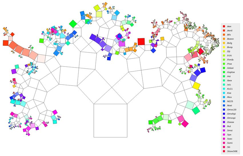
J. Risk Financial Manag. 2020, 13, 309                                                                      4 of 25

     Figure 1 displays the exponentially increasing number of global COVID-19 cases that are
characteristic of the pandemic (at the time of extraction from the Johns Hopkins repository). In May
2020, this highly contagious virus had spread over the five continents of the Earth and infected more
than 4.2 million people in more than 187 countries (out of 198 in total). When writing the paper, the
United States had the highest number of infected individuals, followed by China, Italy, and Iran.
     In the Appendix A, we provide additional insights on this exhaustive database, namely aggregated
data that are ordered by confirmed cases, deaths, recovered cases, and active cases in Tables A1–A4.
Besides, Tables A5–A7 present detailed statistics on the top-10 contributors (by country) in terms of
confirmed cases, deaths, and recovered cases.

2.2. A Susceptible-Infective-Removed (SIR) Model for the World
      In Figure 2, we provide the Susceptible-Infective-Removed (SIR) model by Bailey (1975) for
the World.
      This model supposes that we have a closed, homogeneously mixing population divided into
X (t) susceptible, Y (t) infective, and Z (t) removed individuals at time t. The initial conditions are
set to X (0) = N, Y (0) = a, Z (0) = 0 for some N, a. Because the population is closed, we have
X (t) + Y (t) + Z (t) = N + a for all t ≥ 0, so that the epidemic is completely described by the process
{( X (t), Y (t)), t ≥ 0}. The epidemic is assumed to a continuous-time Markov process on the state space:

                              D N,a = {( x, y) ∈ Z2 : 0 ≤ x ≤ N, y ≥ 0, x + y ≤ N + a}                         (1)

      Transition probabilities are given by:

             Pr (( X (t + δt)), Y (t + δt)) = ( x − 1, y + 1)|( X (t), Y (t)) = ( x, y) = βxyδt + ξ (δt),      (2)

                 Pr (( X (t + δt)), Y (t + δt)) = ( x, y − 1)|( X (t), Y (t)) = ( x, y) = γyδt + ξ (δt)        (3)

     All other transitions have probability ξ (δt), and the parameters β > 0, γ > 0, being known
as the infection rate and removal rate, respectively. The process terminates when the number of
infectives becomes zero, which will almost surely happen within finite time. Further mathematical
derivation is covered, for instance, in Clancy (2014). The SIR model has been applied, among others,
by Shamsi et al. (2018) for post-disaster vaccine provision. Table 1 presents the estimated parameters.

                  Table 1. Parameter estimates for the Susceptible-Infective-Removed (SIR) Model.

                            Parameters used to create the SIR model
                            Region:             ALL
                            Time interval to consider: t0 = 1; t1 = 15; t f inal = 90
                            t0 : 2020-01-23     t1 : 2020-02-06
                            Number of days considered for the initial guess: 15
                            Fatality rate: 0.02
                            Population of the region: 7 800 000 000
                            Convergence: Relative Reduction of F ← FACTR × EPSMCH
                            beta                gamma
                            0.6442002           0.3557998
                            R0 = 1.81056940871835
                            Max of infected: 931947691.37 (11.95%)
                            Max nbr of casualties, assuming 2.00% fatality rate: 18638953.83
                            Max reached at day: 57 → 2020-03-20

    According to the estimates, the “peak” of infections stemming from COVID-19 was reached on
3 March 2020, which justifies the 45-day lock-down that was implemented in most industrialized
countries at the time. Figure 2 reflects the likely trends for the evolution of the epidemic.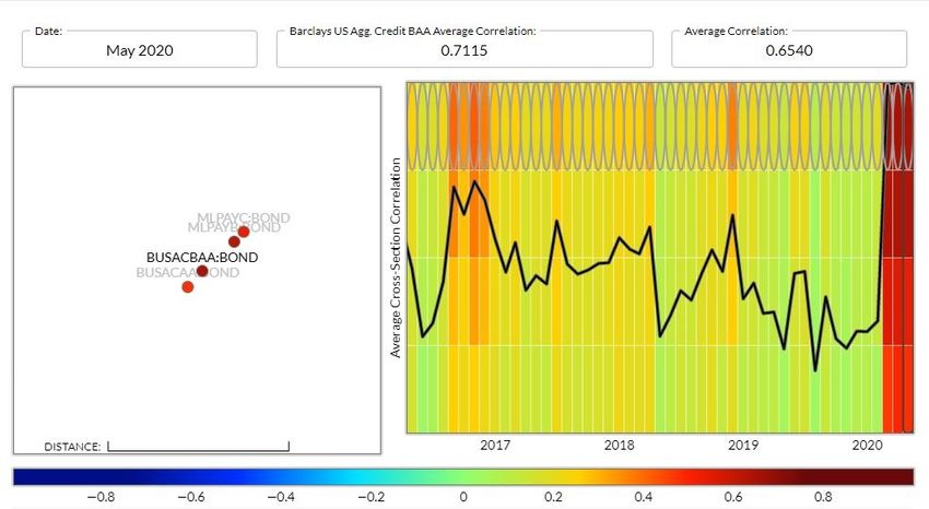
J. Risk Financial Manag. 2020, 13, 309                                                                    5 of 25

The lock-down’s intended effect is to witness a decrease in the contamination level from the COVID-19
and the number of infected.

        Figure 2. SIR Model for the World on all data available from JHU/CCSE repository on 2020-05-05.

    Having covered what medical science can tell us (at the time of writing) regarding the COVID-19
pandemic, we wish to envision how it impacted the world economy in the next section.

3. Asset Markets: The Nightmare Scenario
      At the start of the global Covid-2019 pandemic in 2020, the financial markets entered a period
of enormous financial stress. Corbet et al. (2020) indicate that the volatility relationship between
the main Chinese stock markets and Bitcoin has evolved considerably during this tension period.
Gunay (2020b) finds that the COVID-19 pandemic caused a different and more severe version of the
contagion phenomenon in six different stock markets, such as the United States, Italy, Spain, China, the
United Kingdom, and Turkey. Sharif et al. (2020a) assert that COVID-19 constitutes a significant threat
for the U.S. stock market and carries geopolitical risk. The COVID-19 risk is perceived differently over
the short- and the long-run, and it may be first viewed as an economic crisis.
      The purpose of this section is to establish a quantitative assessment of the economic and financial
consequences of the COVID-19 spreading worldwide, with a statistical assessment of (i) volatility,
(ii) asset allocation, and (iii) risk management.

3.1. A Volatility Perspective
      Things went south very quickly on stock markets. Global stock markets erased approximately
six-trillion U.S. dollars in wealth in one week from 24 to 28 February due to fear and uncertainty
and the rational assessment of investors that firms’ profits are likely to be lower due to the impact of
COVID-19. On 16 March 2020, the Dow Jones plummeted nearly 3000 points. Bonds, oil, and gold
dropped in sync. During the week of 24 March 2020, the S&P 500 experienced its worst week since
the 2008 sub-prime crisis. As can be expected, fear indexes exploded during that period, such as the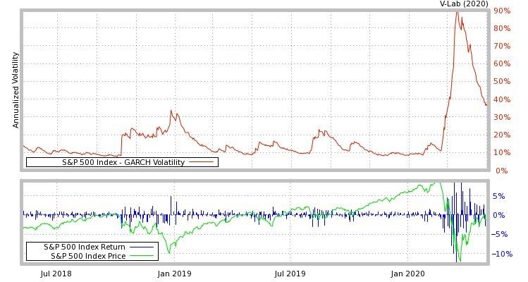
J. Risk Financial Manag. 2020, 13, 309                                                                   6 of 25

VIX (which is computed from options on the S&P 500), or the Financial stress index computed by the
St-Louis Federal Reserve board, which peaked at a year-on-year high (see Figure 3).

      Figure 3. CBOE Volatility Index VIX (top) and St. Louis Fed Financial Stress Index (bottom) from
      2019-05-07 to 2020-05-07. Note: The graph is produced by Board of Governors of the Federal Reserve
      System (US) and the St-Louis Federal Reserve (FRED). VIX: Index, Not Seasonally Adjusted. Frequency:
      Daily, Close. Financial Stress: Index, Not Seasonally Adjusted. Frequency: Weekly, Ending Friday.

     In terms of macroeconomic fundamentals, a severe economic downturn is to be expected.
Its depth can only be foreshadowed based on a preliminary inspection of industrial production data,
which dropped considerablt with the 45-day lock-down that was implemented in most industrialized
countries (see Figure 4). OECD countries, developing countries, and least-developed countries will
experience differentiated impacts. For instance, some countries will be more severely impacted by
others’ closing of trading routes, depending on the price of commodities to be exported to international
trade markets.
     Zhang et al. (2020) have already covered some ground on the COVID-19 sanitary crisis’s financial
aspects. By utilizing graph theory and the minimum spanning tree technique, they map the general
patterns of country-specific risks and systemic risks in the global financial markets. Regional market
integration/collaboration is likely to appear in the face of this major crisis.
     Bae et al. (2003) helps us to define contagion on financial markets by distinguishing between the
terms “Epidemics” (when the virus effects are spread within geographical regions) and “Pandemics”
(when its effects are prevalent across regions). The latter category is characterized by threshold events
of “infection”, similar to what we have witnessed in mid-March 2020. Real and financial consequences
of such outbursts are to be expected.
     The volatility during this window of time goes through the roof (e.g., documented as high
as 49.93% in April 2020 based on a GARCH(1,1) analysis for the S&P 500 index), as presented
in Figure 5. Besides, in Table 2, we verify that all of the parameters are positive and significant.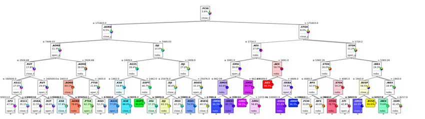
J. Risk Financial Manag. 2020, 13, 309                                                                           7 of 25

According to Bollerslev (1986), the latent volatility process can, indeed, be extracted by modeling
the conditional variance in a Generalized Autoregressive Conditional Heteroskedasticity model:
σt2 = ω + αet2−1 + βσt2−1 . σt2 is the conditional volatility and et2−1 the squared unexpected returns from
previous period. Restrictions apply: ω >0 and α + β < 1. Table 2 contains parameter estimates for
daily volatility. GARCH is now on the dashboard of all asset managers across the industry. The main
parameters of interest are finding positive values (because we are dealing with variances) and statistical
significance. The sum of alpha and beta shall be below unity (otherwise, it indicates the need to estimate
GARCH-variants).

      Figure 4. US Industrial Production Index from 2019-03-01 to 2020-03-01. Note: the graph is produced
      by Board of Governors of the Federal Reserve System (US) and the St-Louis Federal Reserve (FRED).
      Index 2012 = 100. Seasonally Adjusted. Frequency: Monthly.

              Table 2. GARCH(1,1) Parameter estimates and Volatility analysis for the S&P 500 index.

           Parameter Estimates
                                         param              t-stat
                      ω                  0.0154             18.40
                      α                  0.0934             38.62
                      β                  0.8934            383.26
           Volatility Summary
              Closing Price:             $2868.44        Return:              0.90%      1 Week Pred:   33.14%
            Average Week Vol:             36.17%    Average Month Vol:       49.93%     1 Month Pred:   31.92%
                Min Vol:                   6.90%         Max Vol:            89.88%     6 Month Pred:   26.41%
              Average Vol:                17.70%        Vol of Vol:          23.27%      1 Year Pred:   23.09%
                                  Note: The Estimation period is 2 January 1990 to 1 May 2020.

3.2. An Asset Manager’s Perspective
     For skilled traders in the derivatives markets, this pandemic might provide them opportunities to
enhance their Profit & Loss statement. However, for most pension funds, mutual fund investors, and
risk managers, there is “no place to hide” (Buraschi et al. 2014) in the cross-section of returns when
dealing with conventional asset markets (e.g., stocks, bonds, foreign exchange, commodities) or even
with gold Exchange-Traded funds.
     Figure 6 documents an unprecedentedly high level of correlation among international equities,
peaking at 88.93% in April 2020, thereby strengthening the contagion scenario. Correlation analysis
runs by construction from (−1) in blue to (+1) in red. There are opportunities for uncorrelated
investment for the asset manager whenever the blue color is present (which is what he is looking for
according to Markowitz portfolio theory). Only correlated market movements appear in the current
context, which means that the asset manager has no solution to transfer his funds.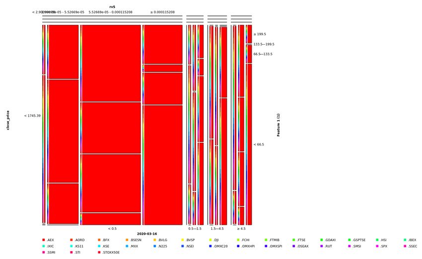
J. Risk Financial Manag. 2020, 13, 309 8 of 25
According to Engle and Sheppard (2001), correlations among assets can be captured through a
Dynamic Conditional Correlation model. A general dynamic correlation structure follows:
1 −1
Qt = S ◦ (ii0 − A − B) + A ◦ Zt−1 Zt0−1 + B ◦ Qt−1 ; Rt = diag{ Qt }− 2 Qt diag{ Qt 2 } (4)
where S is the unconditional variance of the standardized residuals. i is a vector of ones. ◦ is the
Hadamard product of two identically sized matrices. If A, B, and ii0 − A − B are positive semi-definite,
then Q will be positive semi-definite. Rt is the time-varying correlation matrix.
Figure 5. Volatility Analysis for the S&P 500 index as extracted from GARCH(1,1). Note: The graph is
produced by NYU Volatility Lab. The Estimation period is 2 January 1990 to 1 May 2020.
In Table 3, we verify that the DCC(1,1) correlation parameters are all positive and statistically
significant. Table 3 presents correlation estimates (not volatility). We are interested in recovering
statistically significant estimates with a sum of alpha and beta below one (otherwise, misspecification
tests are required). The DCC matrix gives the level of correlation. In our case, it displays an all-time
high correlation level of 88% across asset markets (henceforth, our research question of contagion due
to the COVID-19 pandemic).
In the Appendix A, the interested reader may observe that the picture is the same across other asset
markets (e.g., historical peak in correlations recorded for bonds and commodities in Figures A1 and A2).
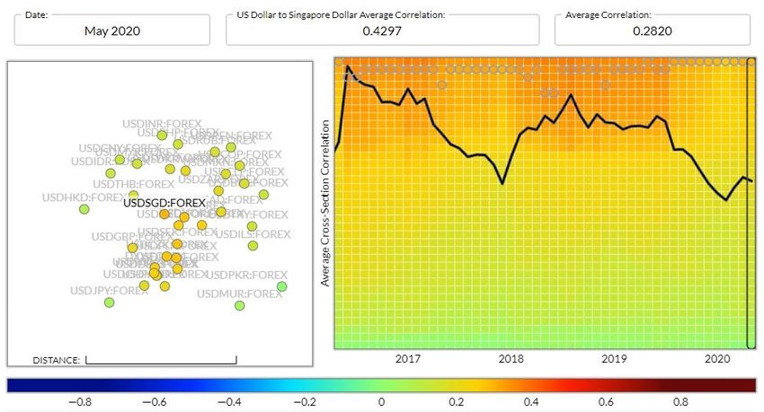
Foreign exchange markets are “frozen” due to the halt of international trade routes (i.e., the correlation
is decreasing in Figure A3).
Table 3. DCC(1,1) Parameter estimates and Correlation analysis.
Parameter estimates
param t-stat
α 0.0096 29.69
β 0.9832 1456.52
Correlation Summary Table
Lower Corr: 0.4739
Upper Corr: 0.8893
1st Factor: 0.7562
2nd Factor: 0.0446
Note: The Estimation period is 15 April 2003 to 1 May 2020.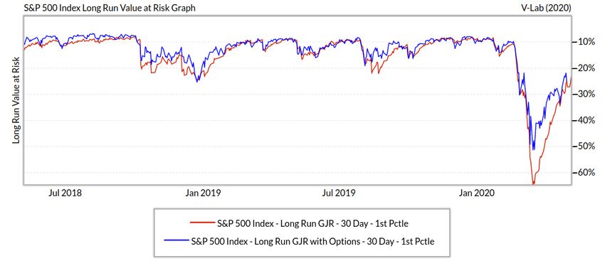
J. Risk Financial Manag. 2020, 13, 309                                                                            9 of 25

      Figure 6. Correlation Analysis for International Equities as extracted from DCC(1,1). Note: The graph
      is produced by NYU Volatility Lab. The Estimation period is 15 April 2003 to 1 May 2020.
      The International Equities dataset contains the following series: iShares MSCI Australia ETF (EWA)
      iShares MSCI Belgium Capped ETF (EWK) iShares MSCI Brazil Capped ETF (EWZ) iShares MSCI
      Canada ETF (EWC) iShares MSCI EAFE ETF (EFA) iShares MSCI Emerging Markets ETF (EEM)
      iShares MSCI Germany ETF (EWG) iShares MSCI Hong Kong ETF (EWH) iShares MSCI Italy Capped
      ETF (EWI) iShares MSCI Japan ETF (EWJ) iShares MSCI Mexico Capped ETF (EWW) iShares MSCI
      Netherlands ETF (EWN) iShares MSCI Singapore Capped ETF (EWS) iShares MSCI Spain Capped
      ETF (EWP) iShares MSCI Sweden Capped ETF (EWD) iShares MSCI Switzerland Capped ETF (EWL)
      iShares MSCI Taiwan Capped ETF (EWT) iShares MSCI United Kingdom ETF (EWU) MSCI Asia Pacific
      (MXAP) MSCI Chile (MXCL) MSCI Europe (MXEU) MSCI USA (MXUS) MSCI World (MXWD) S&P
      500 Index (SPX).

     For digital assets, such as Bitcoin, the deep price plunge that followed the aftermath of the S&P 500
market crash (as illustrated in Figure 7) tells us that they cannot be deemed as a store for value either.
The correlation coefficient between SP500 and CBBTCUSD is computed as 0.83 since the beginning of
the year 20208 . Hence, the popular wisdom that “cash is king” seems to currently prevail.

3.3. A Risk-Manager’s Perspective
     The Value-at-Risk (VaR), a that was concept popularized by Jorion (2000)9 , has also known a
“black-swan” (Taleb 2007) event during March–April 2020, with virtually all holdings from liquidity
risks passing below the 5% threshold usually retained by risk managers. The realization of such an
important risk measure from a risk management perspective is visible in Figure 8.
     This all circles back to the notion of systemic risk that is caused by the pandemic. Systemic
risk refers to the disruption of an economy’s financial system’s proper functioning emanating from
shocks from within or outside the financial system (Martínez-Jaramillo et al. 2010). While numerous
policymakers are exploring the pandemic’s economic impact, lessons that are learned from the global
financial crisis demand the evaluation of financial stability concerning the effective management of the

8   Spearman rank correlation is equal to 0.84, and Kendall’s tau is equal to 0.66.
9   The single-period (n = 1) 1$ VaR on percentage basis is defined by VaR%                 %                       %
                                                                               α = zα σ. VaR95% = (−1.645) σ and VaR99% =
    (−2.33)σ denote its 95% and 99% levels.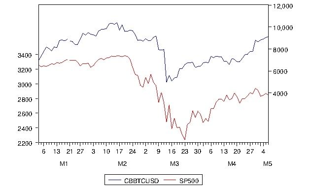
J. Risk Financial Manag. 2020, 13, 309                                                                       10 of 25

pandemic and economy (Cukierman 2011). In the next section, we proceed to algorithmic processing
of COVID-19 and financial data based on operational research techniques.

      Figure 7. Price path of S&P 500 (left Y-axis) contrasted to that of Coinbase Bitcoin Price (right Y-axis)
      during the year 2020 in US $. Note: The data are sourced from St-Louis Federal Reserve Board (FRED).
      The Estimation period is 1 January 2020 to 6 May 2020. SP500 is the S&P 500, Index, Daily, Not
      Seasonally Adjusted. CBBTCUSD is the Coinbase Bitcoin, U.S. Dollars, Daily, Not Seasonally Adjusted.
      Both series are collected with a daily frequency.

      Figure 8. Value-at-Risk for S&P 500 computed either drom daily returns (in red) or from option prices
      (in blue). Note: the graph is produced by NYU Volatility Lab. The Estimation period is 8 May 2018 to
      5 May 2020.

4. Linking the Disease to Predicted Economic Downturn
     Data science comes in handy when in need for analyzing large chunks of data, as is the case with
the depth of the epidemiological and clinical cases on COVID-19 on the one hand, and the heavy
burden put on the servers by high-frequency financial data on the other hand.
     We extract three main time-series for the world from the Johns Hopkins Coronavirus
Center repository:

1.    “ts-confirmed”: time data of confirmed cases,
2.    “ts-deaths”: time series data of fatal cases, and
3.    “ts-recovered”: time series data of recovered cases.
J. Risk Financial Manag. 2020, 13, 309 11 of 25
These series have been thoroughly sourced by Section 2, and further documented in the
Appendix A. We wish to reconstitute the series of events that stemmed from the COVID-19 outbreak
to contagious effects on worldwide stock markets.
For this purpose, we encompass the closing returns from 31 stock markets based on the Oxford
’Realized Library’ with an intra-daily frequency that reaches millions of transactions (2,587,175 at the
time of accessing it). Tick-by-tick data are sampled over the five-minute horizon in order to avoid
microstructure noise (see Barndorff-Nielsen et al. (2008) for the theory). Table 4 details the list of assets.
As a preliminary step, both databases of COVID-19 epidemiological cases and high-frequency
financial data are merged by the time index.
4.1. Hierarchical Decision Tree for Visualizing the Influence of “ts-Confirmed” on Worldwide Stock Markets
In this section, we mobilize a tree algorithm with forward pruning (Breiman et al. 1984;
Quinlan 1986; Smith and Nau 1994) in order to connect the epidemiological cases of COVID-19
(Section 2) to the downward market trends that were observed on stock markets (Section 3).
To feed the decision tree algorithm with stationary data, (i) COVID-19 cases are transformed to
first-differences; and, (ii) stock markets data are transformed to log-returns.10 This pre-processing step
will allow for efficient splitting criteria.
The tree algorithm splits the merged data into nodes by class purity, with “COVID-19 cases” as
the source and “Stock markets” returns as targets. Formally, let us write an adaptive basis-function
model:
M M
f (x) = E[y|x] = ∑ wm I(x ∈ Rm ) = ∑ wm φ(x; vm ) (5)
m =1 m =1
where Rm is the m’th region and wm is the mean response in this region. vm encodes the choice
of variable to split on, and the threshold value, on the path from the root to the m’th leaf.
The basis functions define the regions, and the weights specify the response values in each region
(see Breiman et al. (1984); Quinlan (1986) for an introduction).
Use the following split function to find the optimal partitioning of the data:
( j∗ , t∗ ) = arg min min cost({xi , yi : xij ≤ t}) + cost({xi , yi : xij > t}) (6)
j∈{1,...,D } t∈T j
with T j the set of possible thresholds for feature j by sorting the unique values of xij to a numeric value
t. The most common approach is to consider splits xij = ck or xij 6= ck for each class label ck .
When growing a decision tree, we can prevent over-fitting if the extra complexity of adding an
extra sub-tree is not justified. The standard approach is to grow a “full” tree, and then to perform
pruning. This methodological approach prevents data fragmentation, i.e., too little data fall into
each sub-tree.
In order to determine how far to prune back, the scheme is to evaluate the branches on each
sub-tree and pick the tree that gives the least increase in the chosen statistical error. To measure the
quality of a split, we can resort to:
1
|D| i∑
(i) a multinoulli model π̂c = I(yi = c) with D the data in the leaf by estimating
∈D
class-conditional probabilities,
(ii) a misclassification rate by defining the most probable class label ŷc = arg maxc π̂c and the
1
|D| i∑
corresponding error rate I(yi 6= ŷ) = 1 − π̂ŷ ,
∈D
10 We can transmit unit root tests to interested readers to ensure that the series is I (1) as such.J. Risk Financial Manag. 2020, 13, 309 12 of 25
C
(iii) minimizing the entropy between the test leaf data and class label H(ß̂) = − ∑ π̂c log π̂c , (or
c =1
maximizing the information gain, see, e.g., Quinlan (1987)), or
C
(iv) a Gini index ∑ π̂c (1 − π̂c ) = ∑ π̂c − ∑ π̂c2 = 1 − ∑ π̂c2 , with π̂c the probability of a random
c =1 c c c
entry in the leaf belongs to the class c, and (1 − π̂c ) the probability of mis-classification.
In this paper, we favor cross-entropy and Gini measures.
Table 4. Oxford-Man’s Realized Library: Database Statistics.
Symbol Name Earliest Available Latest Available
.AEX AEX index 3 January 2000 8 May 2020
.AORD All Ordinaries 4 January 2000 8 May 2020
.BFX Bell 20 Index 3 January 2000 8 May 2020
.BSESN S&P BSE Sensex 3 January 2000 8 May 2020
.BVLG PSI All-Share Index 15 October 2012 8 May 2020
.BVSP BVSP BOVESPA Index 3 January 2000 8 May 2020
.DJI Dow Jones Industrial Average 3 January 2000 8 May 2020
.FCHI CAC 40 3 January 2000 8 May 2020
.FTMIB FTSE MIB 1 June 2009 8 May 2020
.FTSE FTSE 100 4 January 2000 7 May 2020
.GDAXI DAX 3 January 2000 8 May 2020
.GSPTSE S&P/TSX Composite index 2 May 2002 8 May 2020
.HSI HANG SENG Index 3 January 2000 8 May 2020
.IBEX IBEX 35 Index 3 January 2000 8 May 2020
.IXIC Nasdaq 100 3 January 2000 8 May 2020
.KS11 Korea Composite Stock Price Index (KOSPI) 4 January 2000 8 May 2020
.KSE Karachi SE 100 Index 3 January 2000 8 May 2020
.MXX IPC Mexico 3 January 2000 8 May 2020
.N225 Nikkei 225 2 February 2000 8 May 2020
.NSEI NIFTY 50 3 January 2000 8 May 2020
.OMXC20 OMX Copenhagen 20 Index 3 October 2005 7 May 2020
.OMXHPI OMX Helsinki All Share Index 3 October 2005 8 May 2020
.OMXSPI OMX Stockholm All Share Index 3 October 2005 8 May 2020
.OSEAX Oslo Exchange All-share Index 3 September 2001 8 May 2020
.RUT Russel 2000 3 January 2000 8 May 2020
.SMSI Madrid General Index 4 July 2005 8 May 2020
.SPX S&P 500 Index 3 January 2000 8 May 2020
.SSEC Shanghai Composite Index 4 January 2000 8 May 2020
.SSMI Swiss Stock Market Index 4 January 2000 8 May 2020
.STI Straits Times Index 3 January 2000 8 May 2020
.STOXX50E EURO STOXX 50 3 January 2000 8 May 2020
Figure 9 shows the result of the COVID-19 pandemic, as measured by the confirmed cases
worldwide, on stock markets’ panic during 2020-01-22 to 2020-05-05 (when last accessed the JHU
repository at the time of writing the paper). Figure 9 shows the connection between financial markets.
At the top of the tree is the financial market from which the contagion stems at the beginning of the
health crisis. At the bottom of the tree, we find spillovers from the original contagion effect.
The resulting tree and decision boundaries are quite complex, even with prunning. The “top”
stock market from which the COVID-19 pandemic spread is detected to be the French CAC 40 indexJ. Risk Financial Manag. 2020, 13, 309 13 of 25
due to the hierarchical nature of the tree-growing process (FCHI, perhaps due to the announcement of
the French president to lock-down the country on 16 March 2020).
Besides, we identify two main “paths” from which the pandemic spread to other financial markets:
1. On the left-hand side, we have the Australian All Ordinaries index (AORD). From Australia,
financial contagion is then visible on sub-trees navigating through US small caps know as Russel
2000 (RUT), the Korean Kospi index (JS11), the UK FTSE, and then at the bottom of the tree
reaching India’s NIFTY 50 (NSEI), Pakistan’s Stock Exchange (KSE), the US Standard & Poor’s
500 (SPX) or the Japanese NIKKEI (N225). Stemming from the overarching “top” of France
and first “branch” Australia, we notice as well other sub-trees channeling though the US Dow
Jones Industrial Average (DJI) with more pronounced regional effects on Canada’s (GSPTSE) and
Mexico’s (MXX) stock exchanges until we reach the bottom of the tree.
2. On the right-hand side, we identify the EURO STOXX 50 (STOXX50E). Contagion occurs
immediately on the first sub-tree on the Amsterdam stock exchange (AEX) with spillovers
in Switzerland (SSMI), Sweden (OMXSPI), and Norway (OSEAX), until Denmark (OMXC20)
at the bottom of the tree. On the second sub-tree (far right of Figure 9), we visualize that the
financial crisis ultimately reaches other European countries, such as Spain (IBEX), Belgium (BFX),
and Finland (OMXHPI). Inter-regional spillovers to Brazil (BVSP, through Spain) and Singapore
(STI, through EURO STOXX) are also visible at the bottom of the tree.
This first strand of the result suggests that contagion first occurred on European and Australasian
stock markets, as the number of COVID-19 confirmed cases was precisely documented and raised
swift public policy responses. If, instead, we plug in the time series “ts-deaths” or “ts-recovered”, we
verify that the decision tree that is reproduced in Figure 9 is stable, i.e., small changes to the input data
(of the same information content) do not have substantial effects on the structure of the tree.11
4.2. Experimenting Mosaic Plots with the Series “ts-Death” on 2020-03-16
Next, in Figure 10 we inspect a Mosaic plot for the day 2020-03-16 that seemed so important as
to place France at the top of the hierarchical tree. Recall that the French president implemented a
45-day lock-down of the country on that date, which seems from our preliminary data analysis to have
wreaked havoc on financial markets.
Mosaic graphs allow visualizing data across two or more dimensions. They are handy when
attempting to capture the relationships between different variables, as in our setting. The Mosaic plot’s
statistical analysis as a contingency table is covered by Friendly (2002).
In Figure 10, the dimensions we are plotting are the following:
• bottom: date chosen for the Mosaic is specifically 2020-03-16;
• left: closing daily prices for stock markets;
• top: intra-day transactions on stock markets; and,
• right: number of deaths reported worldwide on that day according to JHU/CCSE repository.
11 For the sake of brevity, corresponding trees for “ts-deaths” and “ts-recovered” has been saved to disk and can be sent
upon request.J. Risk Financial Manag. 2020, 13, 309 14 of 25
Figure 9. Tree for Origin “ts-confirmed” and Target “Stock markets”. Note: The origin of the tree is COVID-19 confirmed cases worldwide. The Estimation period is
22 January 2020 to 5 May 2020. The first column of Table 4 provides tickers for Stock markets.J. Risk Financial Manag. 2020, 13, 309 15 of 25
Figure 10. Mosaic plot on 2020-03-16 for series “ts-death” and “Stock markets”.J. Risk Financial Manag. 2020, 13, 309 16 of 25
The end result unequivocally paints a “red” picture of how the pandemic, and the incredibly
worrying trend in deaths worldwide, has spread to financial markets, with some of them even briefly
suspending trading (such as the NYSE) during these troubling events. This picture illustrates perfectly,
that, in our opinion, for money managers in such a contagious financial environment with spillovers
of downward closing prices on each stock market, there is “no place to hide”. Had we found other
colors predominant on the Mosaic (e.g., shades of blue or green), we could have advised moving the
funds safely here or there, but there is not such a place (other candidates “safe-havens”, such as Gold
or even Bitcoin, have been discussed in Section 3).
To grasp the meaning of Figure 10 visually, the reader can view it as a carpet plot linking returns
on financial markets. Usually, when such a plot is posted on Twitter about Wall Street blue chips, it
shows the extent to how a piece of news (say, the Boeing 737 MAX industrial disaster) has expanded
into stock markets. They are usually in a net winners or net losers situation. Against the COVID-19
pandemic, what Figure 10 shows, is that there are only losers on financial markets in such circumstances,
highlighting the fact mentioned in the previous Section that there is no place to hide for asset managers
to build alpha strategies.
4.3. A Final Look at the Pythagorean Forest of Influence of “ts-Recovered” on Stock Markets
If we seek to end this paper on a more positive outlook, then we might move the decision tree
upside-down and present it as a forest. To that end, we employ the series “ts-recovered”, which should
be a reason for “rebirth” for the economy, as some patients naturally heal from the COVID-19 (in the
absence of effective treatment at the time of writing, waiting for clinical experiments from Pfizer and
Moderna vaccines).
In Figure 11, we reproduce a Pythagorean Forest, which visualizes how from the tree trunk of
“ts-recovered” new branches and leaves can grow back on financial markets. The Pythagorean Forest
stems from a decision tree model, called “random forest”, where each visualization pertains to one
randomly constructed tree. Its construction is covered by Beck et al. (2014).
Without loss of generality, consider Pythagorean Trees ( Hv , S) :, where Hv = (V, E) is a binary
hierarchy of V = {v1 , . . . , vk } set of k vertices and E ⊂ V × V finite set of edges. S = (c, ∆s, θ ) is
the initial square with center c, length of the sides ∆s, and slope angle θ. The recursive procedure
first draws square S and proceeds if the current hierarchy still contains more than a single node.
Subsequently, encoding the node weights in the squares’ size, the angles α and β are computed
according to the normalized weight of the node opposed to the angle. The width ∆xi of a rectangle Ri
can be changed by modifying the corresponding angle αi accordingly. It should reflect weight wx (vi )
of a vertex vi in relation to the weight of its siblings:
w x ( vi )
αi : = π × n (7)
∑ wx (v j )
j =1
αj
The width of the rectangle is ∆xi := ∆x × sin , where ∆x is the width of the parent node.
2
A maximum branching factor can be implemented. The human reader automatically connects the
rectangles on the curve, which is denoted as the law of continuation.
Figure 11 represents another kind of tree: a “forest”, so to speak since we are concerned here with
patients that recovered from the COVID-19. The goal is to show by a myriad of colors how the increased
number of healing is being transmitted to the various stock markets in the database under increased market
gains. Although being complex to construct, such fractal images exhibit aesthetic properties, which makes
these images easier to interpret. The Pythagorean Forest emphasizes the influence of the root—which is
“ts-recovered”—and its hierarchical influence on subsets down to the level of unitary stock markets. The root
node fills the graph with white color. Its immediate descendants can be understood as higher-level nodes of
the forest.J. Risk Financial Manag. 2020, 13, 309 17 of 25
The image shows that, among the leading directories, the most meaningful parent-child relationships
are to be found with the EURO STOXX 50 (Stoxx50E) in red color; the Amsterdam (AEX), Brussels (BFX),
and Australian (AORD) stock markets in orange color; the French CAC 40 (FCHI) and Dow Jones Industrial
Average (DJI) in light green color; and, the Nordic stock markets of Copenhagen, Helsinki, and Stockholm
(OMXC20, OMXHPI, OMXSPI) in purple colors. This finding confirms the decision tree based on
“ts-confirmed”, where we dated back the origins of the financial contagion to European and Australasian
market, and the U.S. as a repercussion of lock-down implemented in these countries beforehand.
If we move away from the most prominent nodes to the forest’s secondary level, then we can notice
other sub-vertices, each displaying their own set of edges. The granularity of the results obtained with this
visualization tool is remarkable without zooming too much into detail. It is perceptible how the world
economy can “heal” from the Coronavirus as more patients recover from it down to the level of individual
stock markets. For instance, on the forest’s right-hand side, we can see the effects of recovering Amsterdam
or Brussels stock exchanges on the Milan or Frankfurt market places (FTMIB and GDAXI, respectively,
in light green)—hence, these nodes are connected in the sub-hierarchy of the forest.
Overall, we gained an overview of the main branches connecting the COVID-19 epidemiological
cases to the world stock markets. This result’s beauty is that we achieved it without restricting, a-priori,
the number of vertices (e.g., arbitrary hierarchies are allowed).
To further explain our results intuitively, we point out that asset markets are susceptible to
the news. Whenever pharmaceutical companies, like Pfizer, or start-ups, like Moderna, announce
95% of positive results on their COVID-19 vaccines, the financial markets react very positively
with day-to-day increased returns. In our sample, the intuition is that COVID-19 cases are quickly
developing worldwide, which incites stock markets to decline and be linked altogether into a recession
circle. However, the extra data-science experiment illustrates that the global economy can be seen as a
tree whose leaf can become green again (as patients heal, or the vaccine will be mass-administered).
Therefore, financial contagion would bring a new virtuous circle of prosperous economic growth in
the globalized economy.
Figure 11. Pythagorean forest for series “ts-recovered” and “Stock markets”. Note: the origin of the
forest is COVID-19 recovered cases worldwide. The estimation period is 22 January to 5 May 2020.
Tickers for Stock markets are given in the first column of Table 4.J. Risk Financial Manag. 2020, 13, 309 18 of 25
5. Concluding Remarks
As a proteiform disease, COVID-19 is drowning the macro-financial environment into a recession
that it is too early to foreshadow. All in all, confronting several stakeholders’ views amid the COVID-19
outbreak has brought this research a myriad of facts. By merging health and stock market databases,
three types of robust scientific methods have been mobilized in this paper:
1. epidemiological;
2. financial from quants’ viewpoint; and,
3. algorithmic from a data scientist’s viewpoint.
The original contribution is to document the effects of the COVID-19 pandemic on financial
contagion. For the wide dissemination of research results, this paper has opted for a low-key approach
on the technicalities that underlie the models estimated as a methodological choice of the authors.
Whereas decision trees and mosaic plots revealed a heavy concentration of stock markets
plummeting on 16 March 2020 (following a peak of infection detected on 3 March), brighter perspectives
of re-birth: of the economy have been envisioned based on a Pythagorean forest that illustrates the
positive effects of more patients “healing” from the disease.
Given the level of integration of the global financial system, the eminent risk of financial contagion
may further accentuate the global systemic risk. While economies currently at different growth paths
are faced with unique macroeconomic conditions that determine the stability and resilience of their
respective financial systems, the different policy responses that are adopted by different economies in
combating the pandemic will, to a large extent, determine the severity, duration, and management of
both the health and consequent crisis with spillover effects expected (Battiston et al. 2012).
In this regard, while the policy response in one country may help to shield the economy
from domestic adverse economic effects, cross-border financial system interactions may enhance
global financial distress, as vulnerability from one economy is transmitted to other financial systems.
Ultimately, interdependence and the presence of financial contagion mean that the financial system is
as stable as its weakest link.
Therefore, global economies’ ability to effectively manage the impending crisis will depend
on: (i) the effectiveness of individual policy response and (ii) the global financial systems’ ability
to effectively absorb negative spillovers and adverse economic shocks. Systemic risk management
will play a key role in enhancing financial systems’ resilience and providing much-needed financial
intermediation services to the economy. In this regard, continuous analysis and monitoring of the
financial system’s ability remain paramount to realize overall macroeconomic stability (Gunay 2020a).
The study implications relate to the cataclysmic impact of the COVID-19 pandemic on financial
markets. The recession is expected to be severe. Financial contagion is in motion, not only across asset
markets, but also across countries. The ”silver bullet“ to get out of the danger zone would be the swift
deployment of vaccines in the years 2021–22 in order to achieve community resistance to COVID-19.
Regarding future research in this area of banking and finance, the type of data that are needed to
analyze systemic risk and contagion would include (i) individual banks balance sheet and financial
ratios, (ii) cross-sector loans and bonds from financial institutions to the real economy sector, and
(iii) cross border loans and bonds.
The study limitations are based on the restricted data sample at the beginning of the pandemic.
Several years of observations on the consequences of the COVID-19 on global economies will help to
put this first set of results into perspective as data gathering evolves in the scientific community.
Funding: This research received no external funding.
Conflicts of Interest: The author declares no conflict of interest.J. Risk Financial Manag. 2020, 13, 309 19 of 25
Appendix A
Figure A1. Correlation Analysis for Bonds as extracted from DCC(1,1). Note: The graph is produced
by NYU Volatility Lab. The Estimation period is 6 May 1996 to 1 May 2020. The Bonds dataset
contains the following series: Bank of America ML HY Cash Pay B All (MLPAYB) Bank of America
ML HY Cash Pay C All (MLPAYC) Barclays US Agg. Credit AA (BUSACAA) Barclays US Agg. Credit
BAA (BUSACBAA).
Figure A2. Correlation Analysis for Commodities as extracted from DCC(1,1). Note: The graph
is produced by NYU Volatility Lab. The Estimation period is 17 January 2002 to 1 May 2020.
The Commodities dataset contains the following series: CBT-Rough Rice Composite Futures
Continuous (RICE) Gold Spot (GOLD) Lumber, Generic 1st (WOOD) Oats, Generic 1st (OAT) S&P 500
Index (SPX) S&P GSCI Brent Crude Oil Index (BRENT) S&P GSCI Cocoa Index (COCOA) S&P GSCI
Coffee Index (JAVA) S&P GSCI Corn Index (CORN) S&P GSCI Cotton Index (CTN) S&P GSCI Feeder
Cattle Index (FCTL) S&P GSCI Heating Oil Index (HOIL) S&P GSCI Lean Hogs Index (LHOG) S&P
GSCI Live Cattle Index (CATL) S&P GSCI Natural Gas Index (NATGAS) S&P GSCI Platinum Index
(PLAT) S&P GSCI Soybeans Index (SOYB) S&P GSCI Sugar Index (SUGAR) S&P GSCI Wheat Index
(WHEAT) S&P GSCI WTI Crude Oil Index (WTIOIL) Silver Spot (SILV).J. Risk Financial Manag. 2020, 13, 309 20 of 25
Figure A3. Correlation Analysis for Exchange Rates as extracted from DCC(1,1). Note: The graph is
produced by NYU Volatility Lab. The Estimation period is 3 August 2000 to 1 May 2020. The Exchange
Rates dataset contains the following series: United States Dollar Index (DXY) US Dollar to Australian
Dollar (AUD) US Dollar to Brazilian Real (BRL) US Dollar to British Pound (GBP) US Dollar to Canadian
Dollar (CAD) US Dollar to Chilean Peso (CLP) US Dollar to Chinese Renminbi (CNY) US Dollar to
Colombian Peso (COP) US Dollar to Croatian Kuna (HRK) US Dollar to Czech Koruna (CZK) US Dollar
to Danish Krone (DKK) US Dollar to Euro (EUR) US Dollar to Hong Kong Dollar (HKD) US Dollar to
Hungarian Forint (HUF) US Dollar to Indian Rupee (INR) US Dollar to Indonesian Rupiah (IDR) US
Dollar to Israeli Shekel (ILS) US Dollar to Japanese Yen (JPY) US Dollar to Malaysian Ringgit (MYR) US
Dollar to Mauritian Rupee (MUR) US Dollar to Mexican Peso (MXN) US Dollar to Moroccan Dirham
(MAD) US Dollar to New Zealand Dollar (NZD) US Dollar to Norwegian Krone (NOK) US Dollar to
Pakistani Rupee (PKR) US Dollar to Peruvian New Sol (PEN) US Dollar to Philippine Peso (PHP) US
Dollar to Polish Zloty (PLN) US Dollar to Russian Ruble (RUB) US Dollar to Singapore Dollar (SGD)
US Dollar to South African Rand (ZAR) US Dollar to South Korean Won (KRW) US Dollar to Swedish
Krona (SEK) US Dollar to Swiss Franc (CHF) US Dollar to Taiwanese Dollar (TWD) US Dollar to Thai
Baht (THB) US Dollar to Turkish New Lira (TRY).J. Risk Financial Manag. 2020, 13, 309 21 of 25
Table A1. Aggregated Data Ordered By Confirmed Cases available from JHU/CCSE repository on 2020-05-05.
Location Confirmed Perc. Confirmed Deaths Perc. Deaths Recovered Perc. Recovered Active Perc. Active
1 Spain 219,329 5.99 25,613 11.68 123,486 56.30 70,230 32.02
2 Italy 213,013 5.82 29,315 13.76 85,231 40.01 98,467 46.23
3 United Kingdom 194,990 5.32 29,427 15.09 0 0.00 165,563 84.91
4 NYC, NY, USA 176,874 4.83 19,067 10.78 0 0.00 157,807 89.22
5 France 168,935 4.61 25,498 15.09 51,803 30.66 91,634 54.24
6 Germany 167,007 4.56 6993 4.19 135,100 80.89 24,914 14.92
7 Russia 155,370 4.24 1451 0.93 19,865 12.79 134,054 86.28
8 Turkey 129,491 3.54 3520 2.72 73,285 56.59 52,686 40.69
9 Brazil 115,455 3.15 7938 6.88 48,221 41.77 59,296 51.36
10 Iran 99,970 2.73 6340 6.34 80,475 80.50 13,155 13.16
Number of Countries/Regions reported: 187; Number of Cities/Provinces reported: 138; Unique number of distinct geographical locations combined: 3209.
Table A2. Aggregated Data Ordered By Deaths available from JHU/CCSE repository on 2020-05-05.
Location Confirmed Perc. Confirmed Deaths Perc. Deaths Recovered Perc. Recovered Active Perc. Active
1 United Kingdom 194,990 5.32 29,427 15.09 0 0.00 165,563 84.91
2 Italy 213,013 5.82 29,315 13.76 85,231 40.01 98,467 46.23
3 Spain 219,329 5.99 25,613 11.68 123,486 56.30 70,230 32.02
4 France 168,935 4.61 25,498 15.09 51,803 30.66 91,634 54.24
5 NYC, NY, USA 176,874 4.83 19,067 10.78 0 0.00 157,807 89.22
6 Belgium 50,509 1.38 8016 15.87 12,441 24.63 30,052 59.50
7 Brazil 115,455 3.15 7938 6.88 48,221 41.77 59,296 51.36
8 Germany 167,007 4.56 6993 4.19 135,100 80.89 24,914 14.92
9 Iran 99,970 2.73 6340 6.34 80,475 80.50 13,155 13.16
10 Netherlands 41,087 1.12 5168 12.58 0 0.00 35,919 87.42
Number of Countries/Regions reported: 187; Number of Cities/Provinces reported: 138; Unique number of distinct geographical locations combined: 3209.J. Risk Financial Manag. 2020, 13, 309 22 of 25
Table A3. Aggregated Data Ordered By Recovered Cases available from JHU/CCSE repository on 2020-05-05.
Location Confirmed Perc. Confirmed Deaths Perc. Deaths Recovered Perc. Recovered Active Perc. Active
1 Recovered, US 0 0.00 0 NaN 189,791 NaN −160,761 NaN
2 Germany 167,007 4.56 6993 4.19 135,100 80.89 24,914 14.92
3 Spain 219,329 5.99 25,613 11.68 123,486 56.30 70,230 32.02
4 Italy 213,013 5.82 29,315 13.76 85,231 40.01 98,467 46.23
5 Iran 99,970 2.73 6340 6.34 80,475 80.50 13,155 13.16
6 Turkey 129,491 3.54 3520 2.72 73,285 56.59 52,686 40.69
7 China.Hubei 68,128 1.86 4512 6.62 63,616 93.38 0 0.00
8 France 168,935 4.61 25,498 15.09 51,803 30.66 91,634 54.24
9 Brazil 115,455 3.15 7938 6.88 48,221 41.77 59,296 51.36
10 Recovered, Canada 0 0.00 0 NaN 27,006 NaN −27,006 NaN
Number of Countries/Regions reported: 187; Number of Cities/Provinces reported: 138; Unique number of distinct geographical locations combined: 3209.
Table A4. Aggregated Data Ordered By Active Cases available from JHU/CCSE repository on 2020-05-05.
Location Confirmed Perc. Confirmed Deaths Perc. Deaths Recovered Perc. Recovered Active Perc. Active
1 United Kingdom 194,990 5.32 29,427 15.09 0 0.00 165,563 84.91
2 NYC, NY, USA 176,874 4.83 19,067 10.78 0 0.00 157,807 89.22
3 Russia 155,370 4.24 1451 0.93 19,865 12.79 134,054 86.28
4 Italy 213,013 5.82 29,315 13.76 85,231 40.01 98,467 46.23
5 France 168,935 4.61 25,498 15.09 51,803 30.66 91,634 54.24
6 Spain 219,329 5.99 25,613 11.68 123,486 56.30 70,230 32.02
7 Brazil 115,455 3.15 7938 6.88 48,221 41.77 59,296 51.36
8 Turkey 129,491 3.54 3520 2.72 73,285 56.59 52,686 40.69
9 Cook, Illinois, USA 45,223 1.23 1922 4.25 0 0.00 43,301 95.75
10 Netherlands 41,087 1.12 5168 12.58 0 0.00 35,919 87.42
Number of Countries/Regions reported: 187; Number of Cities/Provinces reported: 138; Unique number of distinct geographical locations combined: 3209.J. Risk Financial Manag. 2020, 13, 309 23 of 25
Table A5. Top-ten Contributors to the Time Series of Confirmed Cases available from JHU/CCSE repository on 2020-05-05.
Worldwide ts-Confirmed Totals: 3,662,691
Country. Region Province. State Totals GlobalPerc LastDayChange t−2 t−3 t−7 t − 14 t − 30
1 US 1,204,351 32.88 23,976 22,335 25,501 27,327 28,486 29,515
2 Spain 219,329 5.99 1318 545 884 2144 4211 5029
3 Italy 213,013 5.82 1075 1221 1389 2086 3370 3599
4 United Kingdom 194,990 5.32 4406 3985 4339 4076 4451 3802
5 France 168,935 4.61 1049 614 296 −2512 −2206 3912
6 Germany 167,007 4.56 855 488 697 1627 2357 3251
7 Russia 155,370 4.24 10,102 10,581 10,633 5841 5236 954
8 Turkey 129,491 3.54 1832 1614 1670 2936 3083 3148
9 Brazil 115,455 3.15 6835 6794 4726 6450 2678 1031
10 Iran 99,970 2.73 1323 1223 976 1073 1194 2274
Global Perc, Average: 0.38 (sd: 2.17)
Global Perc. Average in top 10: 7.28 (sd: 9.06)
Number of Countries/Regions reported: 187; Number of Cities/Provinces reported: 83; Unique number of distinct geographical locations combined: 266.
Table A6. Top-ten Contributors to the Time Series of Deaths available from JHU/CCSE repository on 2020-05-05.
Worldwide ts-Deaths Totals: 257,239
Country. Region Province. State Totals GlobalPerc LastDayChange t−2 t−3 t−7 t − 14 t − 30
1 US 71,064 5.90 2142 1240 1313 2612 2326 1519
2 United Kingdom 29,427 15.09 693 288 315 795 837 568
3 Italy 29,315 13.76 236 195 174 323 437 636
4 Spain 25,613 11.68 185 164 164 453 435 700
5 France 25,498 15.09 330 304 135 427 544 833
6 Belgium 8016 15.87 92 80 79 170 264 185
7 Brazil 7938 6.88 571 316 290 430 165 78
8 Germany 6993 4.19 0 127 54 153 246 226
9 Iran 6340 6.34 63 74 47 80 94 136
10 The Netherlands 5168 12.58 86 26 69 145 138 101
Number of Countries/Regions reported: 187; Number of Cities/Provinces reported: 83; Unique number of distinct geographical locations combined: 266.J. Risk Financial Manag. 2020, 13, 309 24 of 25
Table A7. Top-ten Contributors to The time Series of Recovered Cases available from JHU/CCSE
repository on 2020-05-05.
Worldwide ts-Recovered Totals: 1,198,832
Country. Region Province. State Totals LastDayChange t−2 t−3 t−7 t − 14 t − 30
1 US 189,791 2611 7028 4770 4784 2162 2133
2 Germany 135,100 2400 2100 1600 3000 4200 0
3 Spain 123,486 2143 2441 1654 6399 3401 2357
4 Italy 85,231 2352 1225 1740 2311 2943 1022
5 Iran 80,475 1096 957 1072 1352 2148 4500
6 Turkey 73,285 5119 5015 4892 5231 1559 284
7 China.Hubei 63,616 0 0 0 0 5 69
8 France 51,803 1365 465 222 1341 1445 1067
9 Brazil 48,221 2406 2824 2054 1588 2327 0
10 Canada 27,006 976 1109 1107 1096 1266 244
Number of Countries/Regions reported: 187; Number of Cities/Provinces reported: 68; Unique number of
distinct geographical locations combined: 252.
References
Akhtaruzzaman, Md, Sabri Boubaker, and Ahmet Sensoy. 2020. Financial contagion during covid–19 crisis.
Finance Research Letters 101604. [CrossRef]
Al-Awadhi, Abdullah M., Khaled Al-Saifi, Ahmad Al-Awadhi, and Salah Alhamadi. 2020. Death and contagious
infectious diseases: Impact of the covid-19 virus on stock market returns. Journal of Behavioral and Experimental
Finance 27: 100326. [CrossRef] [PubMed]
Andersen, Kristian G., Andrew Rambaut, W. Ian Lipkin, Edward C. Holmes, and Robert F. Garry. 2020.
The proximal origin of sars-cov-2. Nature Medicine 26: 450–52. [CrossRef] [PubMed]
Ashraf, Badar Nadeem. 2020. Stock markets’ reaction to covid-19: Cases or fatalities? Research in International
Business and Finance 101249. [CrossRef]
Bae, Kee-Hong, G. Andrew Karolyi, and Reneé M. Stulz. 2003. A new approach to measuring financial contagion.
The Review of Financial Studies 16: 717–63. [CrossRef]
Bailey, Norman. 1975. The Mathematical Theory of Infectious Diseases. London: Griffin.
Baker, Scott R., Nicholas Bloom, Steven J. Davis, Kyle Kost, Marco Sammon, and Tasaneeya Viratyosin. 2020.
The unprecedented stock market reaction to covid-19. The Review of Asset Pricing Studies 10: 742–58.
[CrossRef]
Barndorff-Nielsen, Ole E., Peter Reinhard Hansen, Asger Lunde, and Neil Shephard. 2008. Designing realized
kernels to measure the ex post variation of equity prices in the presence of noise. Econometrica 76: 1481–536.
Battiston, Stefano, Domenico Delli Gatti, Mauro Gallegati, Bruce Greenwald, and Joseph E. Stiglitz. 2012. Liaisons
dangereuses: Increasing connectivity, risk sharing, and systemic risk. Journal of Economic Dynamics and
Control 36: 1121–41. [CrossRef]
Beck, Fabian, Michael Burch, Tanja Munz, Lorenzo Di Silvestro, and Daniel Weiskopf. 2014. Generalized
pythagoras trees for visualizing hierarchies. Paper presented at 2014 International Conference on Information
Visualization Theory and Applications (IVAPP), Lisbon, Portugal, January 5–8, pp. 17–28.
Bollerslev, Tim. 1986. Generalized autoregressive conditional heteroskedasticity. Journal of Econometrics 31: 307–27.
[CrossRef]
Breiman, Leo, Jerome Friedman, Charles J Stone, and Richard A Olshen. 1984. Classification and Regression Trees.
New York: CRC Press.
Buraschi, Andrea, Robert Kosowski, and Fabio Trojani. 2014. When there is no place to hide: Correlation risk and
the cross-section of hedge fund returns. The Review of Financial Studies 27: 581–616. [CrossRef]
Cheema, Muhammad A., Robert W. Faff, and Kenneth Szulczuk. 2020. The 2008 global financial crisis and
covid-19 pandemic: How safe are the safe haven assets? Covid Economics, Vetted and Real-Time Papers 34:
88–115. [CrossRef]
Clancy, Damian. 2014. Sir epidemic models with general infectious period distribution. Statistics & Probability
Letters 85: 1–5.
Conlon, Thomas, and Richard McGee. 2020. Safe haven or risky hazard? bitcoin during the covid-19 bear market.
Finance Research Letters 35: 101607. [CrossRef] [PubMed]You can also read