Cyber Risk and Cyber Insurance: Actuarial Challenges and Modelling Accumulation Risk with Marked Point Processes
←
→
Page content transcription
If your browser does not render page correctly, please read the page content below
Cyber Risk and Cyber Insurance: Actuarial
Challenges and Modelling Accumulation Risk with
            Marked Point Processes
               based on joint work with Matthias Scherer

                           Gabriela Zeller
                  Technische Universität München
                      Fakultät für Mathematik
                  Lehrstuhl für Finanzmathematik

           DGVFM-eWeiterbildungstag 2021, 18 March 2021
Agenda
text
1. Introduction

2. A Holistic View on Cyber Risk

3. Actuarial Model

4. Simulation Study
5. Conclusion

Gabriela Zeller (TUM) | DGVFM-eWeiterbildungstag 2021 | 18 March 2021   1
Introduction - Academic Literature Review
Numerous contributions from the academic literature divided into:
  • Development of frameworks and taxonomies (e.g. Agrafiotis et al. (2018))
  • Game-theoretic study of interdependent security (e.g. Bolot and Lelarge (2008), Shetty et al.
    (2010))
  • (Empirical) Insurability analysis (e.g. Biener et al. (2015))
  • Modelling of attack rates (stochastic processes, time series analysis) (e.g. Xu et al. (2018))
  • Dependence modelling of attacks (copula approaches) (e.g. Herath and Herath (2011))
  • Models of epidemic spreading on networks (e.g. Fahrenwaldt et al. (2018))
  • Statistical analysis of empirical loss data, often using extreme value theory approaches (e.g.
    Edwards et al. (2016), Eling and Wirfs (2019))

Gabriela Zeller (TUM) | DGVFM-eWeiterbildungstag 2021 | 18 March 2021                                2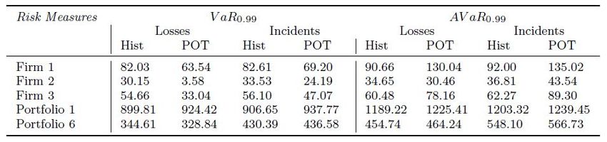
Introduction - Academic Literature Review
Numerous contributions from the academic literature divided into:
  • Development of frameworks and taxonomies (e.g. Agrafiotis et al. (2018))
  • Game-theoretic study of interdependent security (e.g. Bolot and Lelarge (2008), Shetty et al.
    (2010))
  • (Empirical) Insurability analysis (e.g. Biener et al. (2015))
  • Modelling of attack rates (stochastic processes, time series analysis) (e.g. Xu et al. (2018))
  • Dependence modelling of attacks (copula approaches) (e.g. Herath and Herath (2011))
  • Models of epidemic spreading on networks (e.g. Fahrenwaldt et al. (2018))
  • Statistical analysis of empirical loss data, often using extreme value theory approaches (e.g.
    Edwards et al. (2016), Eling and Wirfs (2019))

Summary:
• Cyber risk and insurance much discussed in academia and practice, but:
→ Established modelling approach capturing properties of this new risk type still elusive

Gabriela Zeller (TUM) | DGVFM-eWeiterbildungstag 2021 | 18 March 2021                                2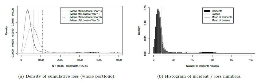
Agenda
text
1. Introduction
2. A Holistic View on Cyber Risk

3. Actuarial Model

4. Simulation Study
5. Conclusion

Gabriela Zeller (TUM) | DGVFM-eWeiterbildungstag 2021 | 18 March 2021   3
Cyber Risk - Definition
Problem: Lack of established definition

Gabriela Zeller (TUM) | DGVFM-eWeiterbildungstag 2021 | 18 March 2021   4
Cyber Risk - Definition
Problem: Lack of established definition
The Geneva Association (2016) suggests the following:

        Any risk emerging from the use of information and communication technology (ICT) that
          compromises the confidentiality, availability, or integrity of data or services.

The definition includes origins,

Gabriela Zeller (TUM) | DGVFM-eWeiterbildungstag 2021 | 18 March 2021                           4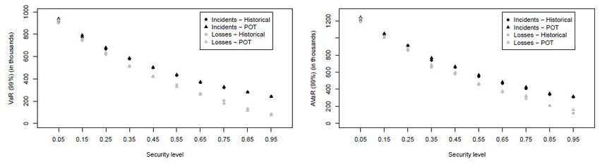
Cyber Risk - Definition
Problem: Lack of established definition
The Geneva Association (2016) suggests the following:

Any risk emerging from the use of information and communication technology (ICT) that compromises
     the confidentiality, availability, or integrity of data or services. The impairment of operational
technology (OT) eventually leads to business disruption, (critical) infrastructure breakdown, and
                              physical damage to humans and property.

The definition includes origins, effects

Gabriela Zeller (TUM) | DGVFM-eWeiterbildungstag 2021 | 18 March 2021                                 4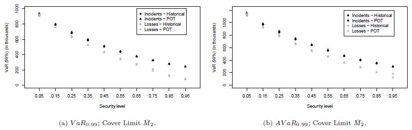
Cyber Risk - Definition
Problem: Lack of established definition
The Geneva Association (2016) suggests the following:

Any risk emerging from the use of information and communication technology (ICT) that compromises
     the confidentiality, availability, or integrity of data or services. The impairment of operational
   technology (OT) eventually leads to business disruption, (critical) infrastructure breakdown, and
  physical damage to humans and property. Cyber risk is either caused naturally or is man-made,
     where the latter can emerge from human failure, cyber criminality (e.g. extortion, fraud),
                                    cyberwar, and cyber terrorism. [...]

The definition includes origins, effects and causes.

Gabriela Zeller (TUM) | DGVFM-eWeiterbildungstag 2021 | 18 March 2021                                 4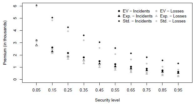
Cyber Risk - Definition
Problem: Lack of established definition
The Geneva Association (2016) suggests the following:

Any risk emerging from the use of information and communication technology (ICT) that compromises
the confidentiality, availability, or integrity of data or services. The impairment of operational technology
 (OT) eventually leads to business disruption, (critical) infrastructure breakdown, and physical damage
  to humans and property. Cyber risk is either caused naturally or is man-made, where the latter can
emerge from human failure, cyber criminality (e.g. extortion, fraud), cyberwar, and cyber terrorism. [...]

The definition includes origins, effects and causes.
→ Cyber risk is dynamic and complex.
→ The application of traditional actuarial approaches faces various challenges.
→ Comprehensive study of cyber risk requires a multitude of perspectives.

Gabriela Zeller (TUM) | DGVFM-eWeiterbildungstag 2021 | 18 March 2021                                      4
Cyber Risk - Key Characteristics
Key challenging properties of cyber risk (Eling and Wirfs (2016), Marotta et al. (2017)):
  • Lack of historical data
  • Dynamic risk type & strategic threat actors
  • Interdependence / accumulation risk
  • Difficult impact determination
  • Information asymmetry (adverse selection / moral hazard) (?)

Gabriela Zeller (TUM) | DGVFM-eWeiterbildungstag 2021 | 18 March 2021                       5
Cyber Risk - Key Characteristics
Key challenging properties of cyber risk (Eling and Wirfs (2016), Marotta et al. (2017)):
  • Lack of historical data
  • Dynamic risk type & strategic threat actors
  • Interdependence / accumulation risk
  • Difficult impact determination
  • Information asymmetry (adverse selection / moral hazard) (?)

Insurability analysis of cyber risk (Biener et al. (2015)):
Most problematic features (in practice) are

  • Lack of independence of loss occurrence
  • Presence of information asymmetries
  • Lack of adequate cover limits

From now on: formal definition of risk as combination of threat, vulnerability and impact.

Gabriela Zeller (TUM) | DGVFM-eWeiterbildungstag 2021 | 18 March 2021                        5
Cyber Risk - Threats
Distinguish threats according to type and root cause:

  • Types are distinguished along their compromise of confidentiality, availability or integrity.
  • Systemic events stem from the existence of a common vulnerability and cause multiple
    simultaneous incidents.
  • Idiosyncratic incidents are connected to the characteristics of the affected / targeted company.

Gabriela Zeller (TUM) | DGVFM-eWeiterbildungstag 2021 | 18 March 2021                                  6
Cyber Risk Model - Company Characteristics Companies are viewed as heterogeneous → different exposure and resilience to identified threats → different impact of a given combination of threat and vulnerability Relevant characteristics: Gabriela Zeller (TUM) | DGVFM-eWeiterbildungstag 2021 | 18 March 2021 7
Agenda
text
1. Introduction

2. A Holistic View on Cyber Risk

3. Actuarial Model

4. Simulation Study
5. Conclusion

Gabriela Zeller (TUM) | DGVFM-eWeiterbildungstag 2021 | 18 March 2021   8
Insurance Portfolio
Assume K insured firms with covariates xj = (xj1 , · · · , xj5 )0 = (bj , sj , dj , cj , nsupj )0 , j ∈ {1, . . . , K }
Examples for covariate ranges:
• Industry sector bj ∈ {FI, HC, BR, EDU, GOV, MAN}
(FI = Finance and Insurance, HC = Healthcare, BR = Business (Retail), EDU = Education,
GOV = Government and Military, MAN = Manufacturing)
• Size sj ∈ {small, medium, large} (by annual revenue and/or number of employees)
• Data dj ∈ {1 = Low risk, 2 = Medium risk, 3 = High risk} (by number of stored records and
whether sensitive data (e.g. PII, PHI) is stored)
• IT Security Level cj ∈ [0, 1] (measured on a standardized scale)
• Number of suppliers nsupj ∈ {1 = Low, 2 = Medium, 3 = High}
→ K × 5 covariate matrix given by
x10
x11 · · · x15
X = ... = ... . . . ... .
xK0 xK 1 · · · xK 5
Gabriela Zeller (TUM) | DGVFM-eWeiterbildungstag 2021 | 18 March 2021 9Excursus: A (Simple) Point Process Gabriela Zeller (TUM) | DGVFM-eWeiterbildungstag 2021 | 18 March 2021 10
Loss Frequency - Idiosyncratic Incidents
Occur independently across firms with rate depending on covariates → simple point processes

Gabriela Zeller (TUM) | DGVFM-eWeiterbildungstag 2021 | 18 March 2021                     11
Loss Frequency - Idiosyncratic Incidents
Occur independently across firms with rate depending on covariates → simple point processes
Specifically, a non-homogeneous Poisson process on [0, ∞) with rate:

                                    λj·,idio (t ) := λ ·,idio (xj , t ) = exp(f· (xj ) + g· (t ))

with · ∈ {DB , BI , FR }, f· (xj ) = αλ ,· + ∑k fλ ,·,k (xjk ) and measurable g· : [0, ∞) → R (standard GAM).

Gabriela Zeller (TUM) | DGVFM-eWeiterbildungstag 2021 | 18 March 2021                                           11
Loss Frequency - Idiosyncratic Incidents
Occur independently across firms with rate depending on covariates → simple point processes
Specifically, a non-homogeneous Poisson process on [0, ∞) with rate:
λj·,idio (t ) := λ ·,idio (xj , t ) = exp(f· (xj ) + g· (t ))
with · ∈ {DB , BI , FR }, f· (xj ) = αλ ,· + ∑k fλ ,·,k (xjk ) and measurable g· : [0, ∞) → R (standard GAM).
For some time point T > 0 let
• NjDB ,idio (T ) be the number of idiosyncratic DBs at firm j during [0, T ]
• N DB ,idio (T ) be the number of idiosyncratic DBs in the whole portfolio during [0, T ]
Gabriela Zeller (TUM) | DGVFM-eWeiterbildungstag 2021 | 18 March 2021 11Loss Frequency - Idiosyncratic Incidents
Occur independently across firms with rate depending on covariates → simple point processes
Specifically, a non-homogeneous Poisson process on [0, ∞) with rate:
λj·,idio (t ) := λ ·,idio (xj , t ) = exp(f· (xj ) + g· (t ))
with · ∈ {DB , BI , FR }, f· (xj ) = αλ ,· + ∑k fλ ,·,k (xjk ) and measurable g· : [0, ∞) → R (standard GAM).
For some time point T > 0 let
• NjDB ,idio (T ) be the number of idiosyncratic DBs at firm j during [0, T ]
• N DB ,idio (T ) be the number of idiosyncratic DBs in the whole portfolio during [0, T ]
I On individual firm level:
Z T
DB ,idio DB ,idio DB ,idio
Nj (T ) ∼ Poi Λj (T ) , where Λj (T ) = λjDB ,idio (t )dt , ∀j ∈ {1, . . . , K }.
0
I On portfolio level (by superposition):
Z T K
DB ,idio
N DB ,idio (T ) ∼ Poi ΛDB ,idio (T ) , where ΛDB ,idio (T ) =
∑ j
λ ( t ) dt .
0 j =1
Gabriela Zeller (TUM) | DGVFM-eWeiterbildungstag 2021 | 18 March 2021 11Loss Frequency - Incidents from Systemic Events Common vulnerability causes multiple simultaneous arrivals → marked point processes Gabriela Zeller (TUM) | DGVFM-eWeiterbildungstag 2021 | 18 March 2021 12
Loss Frequency - Incidents from Systemic Events
Common vulnerability causes multiple simultaneous arrivals → marked point processes
Specifically, start with a non-homogeneous Poisson process Ng· (ground process for the whole
system) with rate:
                                       λ ·,g (t ) = exp(gλ ·,g (t )).
Each arrival of the ground process, {ti }i ∈N , carries a two-dimensional mark with components
                                                 wlog.
                    mi ∈ M := [mmin , mmax ] = [0, 1],                  (strength)
                    Si ∈ S := PK ,                                      (affected subset)

→ marked point process {ti , (mi , Si )0 }i ∈N on [0, ∞) × (M × S ).

Gabriela Zeller (TUM) | DGVFM-eWeiterbildungstag 2021 | 18 March 2021                            12
Loss Frequency - Incidents from Systemic Events
Common vulnerability causes multiple simultaneous arrivals → marked point processes
Specifically, start with a non-homogeneous Poisson process Ng· (ground process for the whole system)
with rate:
λ ·,g (t ) = exp(gλ ·,g (t )).
Each arrival of the ground process, {ti }i ∈N , carries a two-dimensional mark with components
wlog.
mi ∈ M := [mmin , mmax ] = [0, 1], (strength)
Si ∈ S := PK , (affected subset)
→ marked point process {ti , (mi , Si )0 }i ∈N on [0, ∞) × (M × S ).
Assumptions on conditional mark distribution:
• marks {(mi , Si )}i ∈N iid., joint mark distribution independent of location t ∈ [0, ∞)
• mark components {mi }i ∈N and {Si }i ∈N independent
Gabriela Zeller (TUM) | DGVFM-eWeiterbildungstag 2021 | 18 March 2021 12Loss Frequency - Incidents from Systemic Events
Common vulnerability causes multiple simultaneous arrivals → marked point processes
Specifically, start with a non-homogeneous Poisson process Ng· (ground process for the whole system)
with rate:
λ ·,g (t ) = exp(gλ ·,g (t )).
Each arrival of the ground process, {ti }i ∈N , carries a two-dimensional mark with components
wlog.
mi ∈ M := [mmin , mmax ] = [0, 1], (strength)
Si ∈ S := PK , (affected subset)
→ marked point process {ti , (mi , Si )0 }i ∈N on [0, ∞) × (M × S ).
Assumptions on conditional mark distribution:
• marks {(mi , Si )}i ∈N iid., joint mark distribution independent of location t ∈ [0, ∞)
• mark components {mi }i ∈N and {Si }i ∈N independent
Example:
• An event {2, (0.4, {1, 4, 7, 24, 29})} occurs at "timepoint 2", affects firms indexed {1, 4, 7, 24, 29}
across all industries and causes a loss in any of these firms with IT security level < 0.4 (on a
standardized scale)
Gabriela Zeller (TUM) | DGVFM-eWeiterbildungstag 2021 | 18 March 2021 12Loss Frequency - Incidents from Systemic Events
I Event {ti , (mi , Si )0 } reaches firms {j ∈ Si }
I Event {ti , (mi , Si )0 } causes a loss in firms {j ∈ Si , cj < mi } =: {j ∈ Si∗ }
DB Incident DB Loss
DB Incidents DB Losses FR Incident FR Loss
FR Incidents FR Losses BI Incident BI Loss
BI Incidents BI Losses
50
1.0
45
Cyber Incidents in firm j − by sector
0.9
Systemic cyber events − strength
40
0.8
35
0.7
30
0.6
25
0.5
20
0.4
15
0.3
10
0.2
0.1
5
0.0
0
0 1 2 3 4 5 6 7 8 9 10 0 1 2 3 4 5 6 7 8 9 10
Time Time
Gabriela Zeller (TUM) | DGVFM-eWeiterbildungstag 2021 | 18 March 2021 13Loss Frequency - Incidents from Systemic Events
For some time point T > 0 let
DB ,syst
• N̄j (T ) (NjDB ,syst (T )) be the number of systemic DB incidents (losses) at firm j during [0, T ]
• N̄ DB ,syst (T ) (N DB ,syst (T )) be the cumulative number of systemic DB incidents (losses) in the whole
portfolio during [0, T ]
Then, given {ti , (mi , Si )0 }i ∈N and X:
I Individual firm level:
N DB ,g (T )
DB ,syst DB ,g
N̄j (T ) = ∑ 1{j ∈Si } ∼ Poi Λ (t ) · P(j ∈ Si )
i =1
N DB ,g (T )
DB ,syst DB ,g
Nj (T ) = ∑ 1{j ∈Si∗ } ∼ Poi Λ (t ) · P(j ∈ Si ) · P(mi > cj )
i =1
I Portfolio level:
N DB ,g (T )
N̄ DB ,syst (T ) = ∑ |Si |, compound Poisson
i =1
N DB ,g (T )
N DB ,syst (T ) = ∑ |Si∗ | compound Poisson
i =1
Gabriela Zeller (TUM) | DGVFM-eWeiterbildungstag 2021 | 18 March 2021 14Loss Frequency - Incidents from Systemic Events How to choose assumptions for the distribution of |Si | and |Si∗ |? (Translation: Which companies in the portfolio might typically be affected jointly?) • Common vulnerability is often sector-specific I Distinguish between sector-specific events and general events I In either case, assume firms to be affected with equal probability independently from each other → |Si | and |Si∗ | will follow a Binomial mixture distribution Gabriela Zeller (TUM) | DGVFM-eWeiterbildungstag 2021 | 18 March 2021 15
Loss Frequency - Incidents from Systemic Events
How to choose assumptions for the distribution of |Si | and |Si∗ |?
(Translation: Which companies in the portfolio might typically be affected jointly?)
• Common vulnerability is often sector-specific
I Distinguish between sector-specific events and general events
I In either case, assume firms to be affected with equal probability independently from each other

→ |Si | and |Si∗ | will follow a Binomial mixture distribution

Simultaneous arrivals from systemic events allow the model to capture
I lack of independence between cyber losses in a realistic fashion
I overdispersion of claim counts typically found in empirical data
I effect of knowledge about incident / loss in one firm in the portfolio on incident probabilities in
other (similar) firms

Gabriela Zeller (TUM) | DGVFM-eWeiterbildungstag 2021 | 18 March 2021                                   15
Loss Severity
Characteristics of cyber loss severities:
  • Different types of incidents (DB, FR, BI) differ w.r.t. severity distribution
  • Time- and covariate-dependence
  • Typically heavy-tailed, body and tail of distribution modelled separately

Gabriela Zeller (TUM) | DGVFM-eWeiterbildungstag 2021 | 18 March 2021               16
Loss Severity
Characteristics of cyber loss severities:
  • Different types of incidents (DB, FR, BI) differ w.r.t. severity distribution
  • Time- and covariate-dependence
  • Typically heavy-tailed, body and tail of distribution modelled separately

I Promising approach for all types of incidents (Eling and Wirfs (2019)): model cost distribution
directly using a log-normal distribution for the body and a GPD for the tail
Let Lij be the cost of a cyber incident at firm j at time ti , then assume:

             (Lij | Lij ≤ uij· ) ∼ TruncLN µij· , σ · , 0, uij· ,

                                                                        (cyber incidents of daily life)
                           ·             ·    · ·

             (Lij | Lij > uij ) ∼ GPD uij , βij , ξij ,                 (extreme cyber incidents)

where TruncLN (µ, σ , xmin , xmax ) denotes a truncated log-normal distribution on the interval [xmin , xmax ]
and GPD (u , β , ξ ) denotes a generalized Pareto distribution with location u, scale β , and shape ξ .

Gabriela Zeller (TUM) | DGVFM-eWeiterbildungstag 2021 | 18 March 2021                                        16
Loss Severity
Characteristics of cyber loss severities:
• Different types of incidents (DB, FR, BI) differ w.r.t. severity distribution
• Time- and covariate-dependence
• Typically heavy-tailed, body and tail of distribution modelled separately
I Promising approach for all types of incidents (Eling and Wirfs (2019)): model cost distribution
directly using a log-normal distribution for the body and a GPD for the tail
Let Lij be the cost of a cyber incident at firm j at time ti , then assume:
(Lij | Lij ≤ uij· ) ∼ TruncLN µij· , σ · , 0, uij· ,
(cyber incidents of daily life)
· · · ·
(Lij | Lij > uij ) ∼ GPD uij , βij , ξij , (extreme cyber incidents)
where TruncLN (µ, σ , xmin , xmax ) denotes a truncated log-normal distribution on the interval [xmin , xmax ]
and GPD (u , β , ξ ) denotes a generalized Pareto distribution with location u, scale β , and shape ξ .
Alternatives:
• DB: Model severity as number of breached records using log-normal distribution (Edwards et al.
(2016)) and convert into cost of breach using results by Jacobs (2014) or Farkas et al. (2019)
• BI: Use PERT distribution for the body (Hashemi et al. (2015)) and GPD for the tail
Gabriela Zeller (TUM) | DGVFM-eWeiterbildungstag 2021 | 18 March 2021 16Agenda text 1. Introduction 2. A Holistic View on Cyber Risk 3. Actuarial Model 4. Simulation Study 5. Conclusion Gabriela Zeller (TUM) | DGVFM-eWeiterbildungstag 2021 | 18 March 2021 17
Simulation Study - Setting and Loss Distribution
Simulation setting:
  • Fictitious insurance portfolio of K = 500 firms from B = 6 sectors
  • Ten sub-portfolios (K = 50) of equal IT security level
  • T = 5-year observation period, policy duration of one year
  • Uniform distribution of systemic events over sectors
  • Uniform distribution of event strengths
  • Presented results based on 50.000 simulation runs

Gabriela Zeller (TUM) | DGVFM-eWeiterbildungstag 2021 | 18 March 2021    18
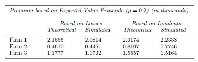
Simulation Study - Results - Premium
I Premiums for three exemplary firms∗

I Premiums according to sub-portfolio losses (equal IT security level)

∗ Firm1: Small manufacturing business with low data risk, supplier risk and IT security, Firm 2: Medium-sized financial company with medium data
and supplier risk and high IT security, Firm 3: Large health care provider with high data risk, medium supplier risk, and average IT security
Gabriela Zeller (TUM) | DGVFM-eWeiterbildungstag 2021 | 18 March 2021                                                                         19
Simulation Study - Results - Risk Measurement
Compare VaR0.99 and AVaR0.99 using the
I Historical estimate
d 1−α (L) = F̂ −1 (1 − α) = L(i ) ,
VaR L
n
\ 1−α (L) = 1
AVaR L(j ) ,
n−i +1 ∑
j =i
where L(1) < L(2) < . . . < L(n) are the order statistics of a realisation of losses L = (L1 , . . . , Ln ),
(1 − α) ∈ i −n1 , ni , and F̂ denotes the empirical c.d.f..
I Peak-over-threshold estimate
βˆ α −ξˆ
VaR 1−α (L) = u +
d 0 −1 ,
ξˆ nn
d 1−α +βˆ −ξˆu
VaR
ˆ , if ξˆ < 1,
\ 1−α (L) =
AVaR 1−ξ
if ξˆ ≥ 1,
∞,
assuming that for a large threshold u, the excesses follow a GPD with parameter estimates βˆ and ξˆ
and n0 is the number of threshold exceedances.
Gabriela Zeller (TUM) | DGVFM-eWeiterbildungstag 2021 | 18 March 2021 20Simulation Study - Results - Risk Measurement I Risk measures for three exemplary firms and two sub-portfolios I Risk measures on sub-portfolio level Gabriela Zeller (TUM) | DGVFM-eWeiterbildungstag 2021 | 18 March 2021 21
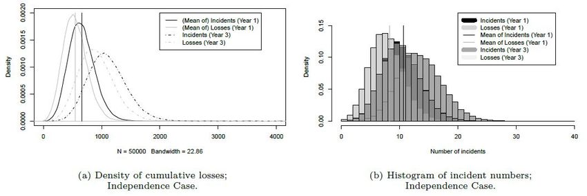
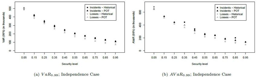
Simulation Study - Results - Accumulation Risk
To emphasize the importance of capturing accumulation risk, compare the case with completely
independent incidents (same marginal frequency for each company, no systemic events)
I Cumulative loss distribution

I Risk measures

Gabriela Zeller (TUM) | DGVFM-eWeiterbildungstag 2021 | 18 March 2021                          22
Simulation Study - Results - Cover Limit
To include realistic policy design and alleviate effects of extremely heavy-tailed severity distributions,
compare to the case with cover limit (truncated loss severities)
I Premium according to sub-portfolio losses

I Risk measures

Gabriela Zeller (TUM) | DGVFM-eWeiterbildungstag 2021 | 18 March 2021                                  23
Agenda
text
1. Introduction

2. A Holistic View on Cyber Risk

3. Actuarial Model

4. Simulation Study
5. Conclusion

Gabriela Zeller (TUM) | DGVFM-eWeiterbildungstag 2021 | 18 March 2021   24
Conclusion
Summary:
  • Cyber risk poses many challenges to traditional actuarial approaches, one of the most severe
    concerns for (re-)insurers being interdependence and resulting accumulation risk
  • The academic literature offers many vantage points on the modelling of cyber risk and
    particularly interdependence, not all of them applicable to real-world portfolios
  • In our view, one of the main sources of interdependence are common vulnerabilities (e.g.
    operating systems, cloud service providers), which may not be easy to understand and diversify in
    a portfolio

Gabriela Zeller (TUM) | DGVFM-eWeiterbildungstag 2021 | 18 March 2021                              25
Conclusion
Summary:
• Cyber risk poses many challenges to traditional actuarial approaches, one of the most severe
concerns for (re-)insurers being interdependence and resulting accumulation risk
• The academic literature offers many vantage points on the modelling of cyber risk and particularly
interdependence, not all of them applicable to real-world portfolios
• In our view, one of the main sources of interdependence are common vulnerabilities (e.g.
operating systems, cloud service providers), which may not be easy to understand and diversify in
a portfolio
Future challenges & chances for academia and practice include:
I Arrangements and standards to facilitate data / information sharing to overcome scarcity of
(publicly) available, reliable data on cyber incidents and related losses
I Interdisciplinary research on properties of cyber risk (mathematical, economic, legal viewpoints)
and continuing cooperations between academia, industry, and government agencies needed
I Design of cyber insurance products that transcend mere risk transfer and promote network
resilience, e.g. by including services using knowledge about portfolio interdependence
Gabriela Zeller (TUM) | DGVFM-eWeiterbildungstag 2021 | 18 March 2021 25Thank you for your attention! Zeller, Gabriela and Scherer, Matthias, A Comprehensive Model for Cyber Risk based on Marked Point Processes and its Application to Insurance (February 12, 2021). Available at SSRN: https://ssrn.com/abstract_id=3668228
References
  • Agrafiotis, I., Nurse, J., Goldsmith, M., Creese, S., and Upton, D. A taxonomy of cyber-harms:
      Defining the impacts of cyber-attacks and understanding how they propagate. Journal of
      Cybersecurity, 4(1), 2018.
  •   Biener, C., Eling, M., and Wirfs, J.H. Insurability of cyber risk: An empirical analysis. The Geneva
      Papers on Risk and Insurance - Issues and Practice, 40(1):131-158, 2015.
  •   Bolot, J. and Lelarge, M. A new perspective on internet security using insurance. In IEEE
      INFOCOM 2008 - The 27th Conference on Computer Communications, p. 1948-1956.
  •   Edwards, B., Hofmeyr, S., and Forrest, S. Hype and heavy tails: A closer look at data breaches.
      Journal of Cybersecurity, 2(1):3-14, 2016.
  •   Eling, M. and Wirfs, J.H. Cyber risk: too big to insure? Risk transfer options for a mercurial risk
      class, Volume 59 of IVW-HSG-Schriftenreihe, 2016.
  •   Eling, M. and Wirfs, J.H. What are the actual costs of cyber risk events? European Journal of
      Operational Research, 272(3):1109-1119, 2019.
  •   Farkas, S., Lopez, O., and Thomas, M. Cyber claim analysis through Generalized Pareto
      Regression Trees with applications to insurance pricing and reserving., 2019.
      https://hal.archives-ouvertes.fr/hal-02118080

Gabriela Zeller (TUM) | DGVFM-eWeiterbildungstag 2021 | 18 March 2021                                    26
References
• Fahrenwaldt, M., Weber, S., and Weske, K. PRICING OF CYBER INSURANCE CONTRACTS IN
A NETWORK MODEL. ASTIN Bulletin, 48(3), 1175-1218, 2018.
• Hashemi, S.J., Ahmed, S., and Khan, F. Probabilistic modeling of business interruption and
reputational losses for process facilities. Process Safety Progress, 34(4):373-382, 2015.
• Herath, H. and Herath, T. Copula-based actuarial model for pricing cyber-insurance policies.
Insurance Markets and Companies, 2(1), 2011.
• Jacobs, J. Analyzing Ponemon cost of data breach.
https://datadrivensecurity.info/blog/posts/2014/Dec/ponemon/, 2014.
• Marotta, A., Martinelli, F., Nanni, S., Orlando, A., and Yautsiukhin, A. Cyber-insurance survey.
Computer Science Review, 24:35-61, 2017.
• Shetty, N., Schwartz, G., Felegyhazi, M., and Walrand, J. Competitive cyber-insurance and
internet security., Economics of Information Security and Privacy, volume 5, p. 229-247, 2010.
• The Geneva Association, Eling, M., and Schnell, W. 2016, Ten Key Questions on Cyber Risk and
Cyber Risk Insurance. https://www.genevaassociation.org/sites/default/les/
research-topics-documenttype/pdf_public/cyber-risk-10_key_questions.pdf, 2016.
• Xu, M., Schweitzer, K., Bateman, R., and Xu, S. Modeling and predicting cyber hacking breaches.,
IEEE Transactions on Information Forensics and Security, 13(11):2856–2871, 2018.
Gabriela Zeller (TUM) | DGVFM-eWeiterbildungstag 2021 | 18 March 2021 27You can also read