Daylight Saving Time and Homicides: Light Effect in Crimes of a Brazilian State Horário de Verão e Homicídios: Efeito da Luz de um Estado Brasileiro

Daylight Saving Time and Homicides: Light Effect in Crimes of a
 Brazilian State

 Horário de Verão e Homicídios: Efeito da Luz de um Estado
 Brasileiro

 Renan Xavier Cortesa
 Adelar Fochezattoa
 Paulo de Andrade Jacintob

Abstract: This article analyzes the effect of daylight saving time (DST) on crimes in
the Brazilian state of Rio Grande do Sul. With the argument that DST provides “more”
hours of light throughout the day, it is expected that the criminal behavior will reduce at
its implantation, since a clearer environment can dissuade the potential criminal. Mak-
ing use of several regression discontinuity design (RDD) models and a daily database
ranging from 2006 to 2014 of the Mortality Information System (SIM) of Datasus, the
models were estimated separately by year, being able to include wheater independent
variables (such as temperature, precipitation and wind speed) and fixed effects of days
of the week. It was evidenced that DST has no significant effect on changes in homicide
rates per 100,000 inhabitants, neither in its beginning, nor its end. On the other hand,
it has been found that, in general, there is a strong weekend effect on criminal activity
and some evidence that homicide rates are related to temperature.

Keywords: Crime. Criminology. Daylight saving time. Homicide rate. Regression dis-
continuity design.

Resumo: Este artigo analisa o efeito do horário de verão (HV) sobre os crimes no es-
tado do Rio Grande do Sul (BR). Com o argumento de que o HV fornece “mais” horas
de luz ao longo do dia, espera-se que o comportamento criminoso diminua na sua
implantação, uma vez que um ambiente mais claro pode dissuadir o potencial crimi-
noso. Utilizando diversos modelos de regressão descontinuidade e um banco de dados
diário de 2006 a 2014 do Sistema de Informações sobre Mortalidade (SIM) do Datasus,
os modelos foram estimados separadamente por ano, podendo incluir variáveis ​​inde-
pendentes de maior temperatura (como temperatura, precipitação e velocidade do
vento) e efeitos fixos de dias da semana. Evidenciou-se que o HV não tem efeito signifi-
cativo na mudança das taxas de homicídio por 100.000 habitantes, nem em seu início,
nem em seu fim. Por outro lado, verificou-se que, em geral, há um forte efeito de fim de
semana sobre a atividade criminosa e algumas evidências de que as taxas de homicídio
estão relacionadas à temperatura.

a Pontifícia Universidade Católica do Rio Grande do Sul (PUCRS), Escola de Negócios, Programa
 de Pós-Graduação em Economia (PPGE). Porto Alegre, Rio Grande do Sul, Brasil.
b Universidade Federal do Paraná, Departamento de Economia (DEPECON). Curitiba, Paraná, Brasil.

 Análise Econômica, Porto Alegre, v. 39, n. 79, p. 7-33, jun. 2021. 7
 DOI: dx.doi.org/10.22456/2176-5456.80052

Palavras-chave: Crime. Criminologia. Horário de verão. Taxa de homicídios. Re-
gressão com descontinuidade.

JEL Classification: C14; Q58; K42.

1 Introduction

 According to the rational choice theory of delinquent behavior from Becker
(1968), the individual chooses to commit a crime if the expected benefits are grea-
ter than the expected costs where several factors influence both incentives. Regar-
ding the expected benefits, criminals can assess the financial return of crime and/
or the psychic return of crime by increasing their utility. On the other hand, costs
considered are planning time, probability of being captured, severity of punish-
ment, moral cost, labor instrument cost (such as a firearm), opportunity cost in the
legal labor market, etc. In this context, the probability of being captured may play
an important deterrent to crime.
 According to Doleac and Sanders (2005), an environment of greater clarity
makes the witnesses more apt to see offenders committing crimes. In other words,
this environment facilitates the identification of criminals by individuals, increasing
the number of potential witnesses and identification of perpetrators in case of sei-
zure. In their model, the expected cost of crime is a function that depends, besides
other factors, on the probability of capture, which depends on the light of the envi-
ronment. Among some papers that relate the clarity of the environment to criminal
activity, we can highlight Salvi (2011), which studied the additional perpetuation of
lights in Los Angeles, and Arvate et al. (2015), who evaluated the Brazilian federal
program Luz para Todos (Light for All) in the rural environment, which found a
reduction in the number of violent crimes.
 One of the ways to assess whether clarity affects criminal behavior is to make
use of daylight saving time (DST). DST consists in advancing the clock one hour
during the months close to summer, making daylight better utilized in the begin-
ning of the night and, consequently, causing ”more” hours of sunlight during the
afternoon. In this sense, society would save energy, with this being its main objec-
tive (ARIES; GUY, 2008). Although time of day plays a very important role in social
organizations, affecting the moment of waking up, working, lunch, sleeping, etc.,
this article justifies its approach under the hypothesis that there is a criminal deter-
rence effect through brightness of the environment.
 Several papers analyze the effect of DST with different objectives. Kountouris
and Remondou (2014) find evidence for Germany that DST has a negative in-
fluence on satisfaction and mood, especially on people who work full time. Smith

8 Análise Econômica, Porto Alegre, v. 39, n. 79, p. 7-33, jun. 2021.

(2016) examines the effect of DST in fatal car accidents pointing that it increases
the risks due to the change in the sleep schedule and the reallocation of morning
light to evening. Toro et al. (2015) also show that the shift to DST has an influence
on the risk of acute myocardial infarction. Kotchen and Grant (2011) find evidence
contrary to the main objective of DST, as their results indicate that there is an ap-
proximately 1% increase in energy consumption for the state of Indiana in the USA.
In addition, Kellogg and Wolff (2008) have no effect on energy consumption in
Australia. In beneficial terms, Wolff and Makino (2012) show that the time spent in
recreation increases during DST, while the time spent at home watching television
decreases and this translates into an additional 10% calorie burn.
 In terms of criminality, Doleac and Sanders (2005), making use of regression
discontinuity design (RDD) and differences-in-differences, evaluate the effects of
change on DST in United States (US) in various crime categories. They estimate
a 7% drop in robberies after the DST beginning and a 11% reduction in rapes, in
addition, they estimate a significant social cost savings through the simple exten-
sion of DST policy in US.
 In Brazil, Toro et al. (2016) analyze the effect of DST in Brazilian states for
firearm deaths, since this type of murder plays an important role in Brazilian crimes
(DE SOUZA et al., 2007). Considering that in Brazil some states adopt the DST
policy and others do not,1 their work, making use of RDDs, difference-in-difference
and differences in discontinuities, analyzed within and between state effects, com-
paring “treated” and “untreated” states. In addition, Toro et al. (2016) estimated
that the change in ambient light caused by the DST was responsible for saving
about 3,850 potential victims from 2006 to 2011.
 Based on these considerations, this article aims to analyze the effect of the
change in DST in homicide cases for the Brazilian state of Rio Grande do Sul (RS)
between the years 2006 and 2014. The study differs in some respects in relation to
Toro et al. (2016). The first, the specific case of a UF, RS, will be evaluated, allowing
a more detailed analysis from the intra-annual point of view, with the inclusion of cli-
matological covariates such as temperature, precipitation and wind speed. This is an
important contribution insofar as in the state of RS, climate changes are well defined.
In addition, there is abundant evidence of the association between climatic variables
and the occurrence of crimes reported in the literature, such as the studies of Cec-
cato (2005) for Brazil, Michel et al. (2016) and Ranson (2014) for the United States,
Horrocks and Menclova (2011) for New Zealand and Tompson and Bowers (2015)
for Scotland. The second, it will also be of interest to evaluate the effect of the exit of
the DST, since this type of intervention is characterized by the reduction of hours of

1 The states that adopts the DST are Rio Grande do Sul, Santa Catarina, Paraná, São Paulo, Rio de
 Janeiro, Espírito Santo, Minas Gerais, Bahia (in 2011), Goiás, Mato Grosso, Mato Grosso do Sul
 and Distrito Federal.

 Análise Econômica, Porto Alegre, v. 39, n. 79, p. 7-33, jun. 2021. 9

sunshine throughout the afternoon. That is, if the number of homicides is expected to
decrease when DST is started, it is reasonable to assume that it will rise as DST ends,
something unheard of in the literature related to the subject.
 The article is structured in five sections besides this introduction. In Section 2
it is presented a review of the Brazilian Energy Policy. Section 3 describes the sour-
ce of the data and the empirical strategy. The results are presented and discussed
in Section 4. Section 5 describes the robustness tests. Section 6 presents the final
considerations. The results show that DST has no significant effect on changes in
homicide rates per 100,000 inhabitants, neither in its beginning, nor its end. Howe-
ver, we found that there is a strong weekend effect on criminal activity and some
evidence that homicide rates are related to temperature.

2 Brazilian Energy Policy

 The DST is a policy that aims to reduce electricity consumption in the eve-
ning, between 6 pm and 9 pm, by making better use of natural light. It was first
adopted in Brazil in 1931, but it was only from 2008 that it became regulated its
obligatoriness. The decree that regulates it establishes the regions in which it takes
effect, the moment it starts each year (midnight on the third Sunday of October)
and the moment it ends (midnight on the third Sunday of the month of February of
the following year). Since then the program has been adopted normally.
 In 2017, a study carried out by the National Electric System Operator and the
Ministry of Mines and Energy pointed out that between 2013 and 2016 the energy
saved decreased from R$ 405 million to R$ 159.5 million per season. The study
says that because of changes in consumer habits, the program no longer has the
same effect in past years in terms of reducing energy consumption at peak times,
leading to a reduction in energy savings. The justification is that there was a shift in
the schedule of higher consumption of electricity, which used to be in the interval
between 17h and 20h and is currently in the interval between 14h and 15h. Due
to this study, in 2017 the government considered ending the program, which did
not happen. The debate is set and goes beyond the technical question of energy sa-
ving, because interested parties, such as producers of drinks, bars and restaurants,
have already expressed their support for the maintenance of the program. This
study, when testing the hypothesis that DST affects crime, is also inserted indirectly
in this debate.

10 Análise Econômica, Porto Alegre, v. 39, n. 79, p. 7-33, jun. 2021.

3 Methodology

 In this section, we detail the data, methodology and design approach used of
this study. We will give a general overview of the data and the mathematical back-
ground for the regression used.

3.1 Data Source

 The Brazilian Ministry of Health through the Mortality Information System
(SIM) has mortality information at the municipal level, including date and time of
death. The SIM is a reliable source of data since it relies on legal certificates of mor-
tality regulated by the federal government. In this database it is possible to identify
the cause of death through the codes of the International Statistical Classification
of Diseases and Related Health Problems (ICD-10). Another database to be used is
one of the National Institute of Meteorology (INMET) which has daily public wea-
ther data for 19 municipalities in Rio Grande do Sul where meteorological stations
are installed. The municipal population data were obtained from the estimates of
the Statistics and Economics Foundation of Rio Grande do Sul (FEE-RS).
 In the field of criminality, due to the reliability level of homicide information,
this is often used to estimate the crime rate of a given region. The homicides com-
mitted with firearms, including also, the homicides caused by sharp, penetrating
and blunt objects will be used. In addition, the occurrence of crimes for undetermi-
ned intent. Table 1 describes the ICD-10 categories used in this work.

Table 1 – Code description of ICD-10 used
 Code Description
 X93 Assault by handgun discharge
 X94 Assault by rifle, shotgun and larger firearm discharge
 X95 Assault by other and unspecified firearm discharge
 X99 Assault by sharp object
 Y00 Assault by blunt object
 Y22 Handgun discharge, undetermined intent
 Y23 Rifle, shotgun and larger firearm discharge, undetermined intent
 Y24 Other and unspecified firearm discharge, undetermined intent

Source: Elaborated by the author.

 An important feature, which is also raised in the work of Toro et al. (2016), is
the relation if the increase in mortality during the hours most affected by the DST
are results of a crime-lagging effect occurring in hours before DST. For example, it
may happen that a victim who has suffered a criminal incident (a shot, for exam-

 Análise Econômica, Porto Alegre, v. 39, n. 79, p. 7-33, jun. 2021. 11

ple) hours before sunset ends up dying in the hospital hours near the DST transi-
tion time. One possible way to try to circumvent this spurious effect is to limit the
study to cases where the victim died at the scene of the crime.2 In this sense, the
analyzes contemplate this characteristic working only with the cases that occurred
outside hospitals or other health establishments.3

3.2 Regression Discontinuity Design

 The RDD or discontinuous regression method can be used when the proba-
bility of receiving a treatment changes discontinuously with a numerical variable.
The idea of this method is to evaluate the effect of an intervention in the surroun-
dings of values “closer” of what was defined as intervention threshold. It is expec-
ted that if there is an effect on the intervention, there will be a discontinuity in
these more critical values since the observational units that will be closer to this
threshold will have greater incentives (or not) to change the values of the depen-
dent variable. With this expected hypothesis, this jump due to the change in status
of receiving treatment can be interpreted as a local average treatment effect. Thus,
this is one of the points that may represent a limitation of the method, since it es-
timates an average effect of the treatment comparing only individuals around this
cut-off point and, therefore, extrapolations to the rest of the population should be
made with caution.
 According to Menezes Filho et al. (2012), one of the first works to introdu-
ce the idea of regression discontinuity was Thistlewaite and Campbell (1960) in
which this method was used to evaluate the impact of a merit award on students’
academic performance. Another application, still in the education economics, can
be seen in Dee and Wyckoff (2013) which used RDD to evaluate performance
and probability of retention of teachers in an evaluation system that had financial
incentives for those with scores above a certain value and threat of dismissal for
teachers with performances below a certain score. In this sense, this study used this
method for two discontinuities: between teachers with threat of dismissal and ave-
rage teachers and another discontinuity between average teachers and teachers
who received financial incentives.
 Specifically, in the case of using the method to evaluate the effect of DST, the
variable that undergoes the intervention is the time measured by the days after the

2 In SIM database, there is a variable of Death Occurrence Location in which it is possible to filter
 by hospital, public road, home, etc.
3 Two important features must be raised in this regard: the first is that this type of filter is more con-
 servative because observations are missed where the victim is injured and is quickly admitted to a
 hospital and dies soon after their admission and, secondly, also excludes those cases in which the
 execution took place inside a hospital. This filter resulted in a reduction of 27.54% of cases, but our
 model proved to be robust regarding this data treatment, as presented in Section 5.5.

12 Análise Econômica, Porto Alegre, v. 39, n. 79, p. 7-33, jun. 2021.

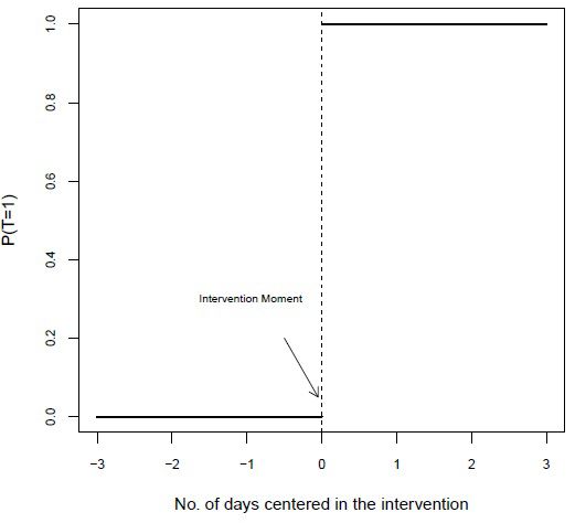
establishment of the DST. With this, the variable takes negative discrete values before
the intervention and discrete positive values after the intervention, assuming the va-
lue zero on the first day after the DST. This type of discontinuous regression is called
the “sharp” type, since the regions have zero probability of participating in the DST
in the days preceding it, but they have probability equal to one after the intervention.
 In order to define the local average treatment effect (LATE), we define a va-
riable of interest , which in our case are the criminal events, a variable , which
are the number of days after the DST, and a constant that determines when the
observational unit will be treated. As defined, in our case this constant will be zero
because it represents exactly the first day after the establishment of the DST. The
LATE is defined as:

 ( ) = [ (1) | – = ] − [ (0) | = ] (1)

 However, it is not possible to observe (1) and (0) for the same region, what is
observed in fact is:

 = (0) – ( (1) − (0)) × (2)

 where = 1 => = (1) and = 0 => = (0). However, a treatment va-
riable depends on a continuous covariable Z which undergoes a discontinuity.
Therefore, the expected value for treated unities (after threshold) is given by:

 [ | = + ] = [ (0)| = + ] + –[( (1) − (0)) × | = + ] (3)

 and for individuals below the threshold (before DST) is given by:

 [ – = − ] = [ (0)– = − ] + –[( (1) − (0)) × – = − ] (4)

 In the sharp case, the switch to treatment is abrupt, where all the observatio-
nal units with a value of above the constant receive the treatment and all the
others do not receive. The LATE is:

 ( ) = + − − = lim [ | = – + ] − lim [ – = − ] (5)

 ↓0 ↓0

 For illustrative purposes, Figure 1 shows this sudden change in treatment
probability shortly after DST change.

 Análise Econômica, Porto Alegre, v. 39, n. 79, p. 7-33, jun. 2021. 13

Figure 1 – Representation of a sharp intervention

Source: Elaborated by the author.

 In terms of modeling, the equation below presents the model in its reduced
form:
 = 0 + ( ≥ 0) + ( ) + + (6)

 where represents the number of days after DST, represent years, is the
horizontal axis variable (also referred as running variable), represents a vector
of covariates, (.) is a flexible function nonparametrically estimated, is the de-
pendent variable which, in this case, is the homicide rate per 100,000 inhabitants
and represents the effect of DST discontinuity on the dependent variable and can
be interpreted as the local effect of the treatment. As in Doleac and Sanders (2005)
and Toro et al. (2016), it is expected that the criminal rate falls more sharply in the
hours most affected by the transition. Thus, models will be estimated by analyzing
both the full day and the hours close to sunset (both before and after). Additionally,
covariables will be included as the day of the week and climatological variables.
 This type of discontinuity regression can be seen as a semiparametric model,
being a particular case of the Generalized Additive Models (GAM) (LOEFFLER;
GRUNWALD, 2015). Thus, its equation will be estimated via GAM, where its
nonparametric function of the variable will be estimated via local linear polyno-
mial regression Loess (CLEVELAND; DEVLIN, 1988) with smoothing parameter
equal to 0.5.

14 Análise Econômica, Porto Alegre, v. 39, n. 79, p. 7-33, jun. 2021.

3.3 Data Preparation

 Before presenting the results obtained, some considerations must be made
regarding the data used in the study. Firstly, to control the possible idiosyncrasies of
the data it is emphasized that models will be estimated with the inclusion of cova-
riables, such as weekdays and daily climatological variables. In addition, this paper
uses homicide rates as dependent variable, that is, it is already corrected by the size
of the population. The climatological variables obtained on the INMET website are
average temperature information,4 wind speed and pluviometric precipitation.5
Considering that INMET presents data only for 19 municipalities where meteorolo-
gical stations are present, the estimated values for RS represent a weighted average
by the population of each of these municipalities.
 Another important fact that is taken into account is that on the day that the DST
begins, clocks must be advanced by one hour and in this sense the day “loses” one
hour which could underestimate the number of homicide cases on the day immedia-
tely following the change in DST. To correct this possible distortion, the number of ho-
micides occurring on this day is multiplied by 24/23.6 Similarly, when DST is terminated
the number of deaths of the immediately subsequent day is multiplied by 23/24.
 The variable that represents the number of days until the start (or end) of DST
is constructed according to Table 2.

Table 2 – DST dates implemented
 Season Duration
 2005/2006 from 0am of October 16, 2005, until 0am of February 19, 2006
 2006/2007 from 0am of November 5, 2006, until 0am of February 25, 2007
 2007/2008 from 0am of October 14, 2007, until 0am of February 17, 2008
 2008/2009 from 0am of October 19, 2008, until 0am of February 15, 2009
 2009/2010 from 0am of October 18, 2009, until 0am of February 21, 2010
 2010/2011 from 0am of October 17, 2010, until 0am of February 20, 2011
 2011/2012 from 0am of October 16, 2011, until 0am of February 26, 2012
 2012/2013 from 0am of October 21, 2012, until 0am of February 17, 2013
 2013/2014 from 0am of October 20, 2013, until 0am of February 16, 2014
 2014/2015 from 0am of October 19, 2014, until 0am of February 22, 2015
 2015/2016 from 0am of October 18, 2015, until 0am of February 21, 2016
Source: Elaborated by the author.

4 In the meteorological stations three temperature readings are made every six hours. For a perfect
 control, a fourth reading should be done, which is not usually the case. Thus, the average tempe-
 rature that is calculated is not exactly the average of the day. What meteorologists do then is to
 calculate an average of the three readings, plus the maximum and the minimum. The average of
 these five values is called average temperature compensated and this is the information used here.
5 Other variables were considered but excluded due to excess of missing data.
6 This correction is also made by Toro et al. (2016) although the results have been robust to it in their
 work.

 Análise Econômica, Porto Alegre, v. 39, n. 79, p. 7-33, jun. 2021. 15

4 Results

 In this section, we present the main descriptive results, as well as the main re-
sults of the analysis. We highlight that we investigated the start and the end of DST.

4.1 Descriptive Statistics

 In this section we analyze some descriptive statistics of the SIM database for
Rio Grande do Sul in the period between 2006 and 2014. Figure 2 shows daily
homicide rates per 100 thousand inhabitants stratified per year. We see that the va-
lues oscillate near 0.04 with some outliers surpassing the values of 0.12. In addition,
there is no specific year that distinguishes itself from others in level terms. On the
horizontal axis of each these graphs are the number of days in relation to the start
day of DST (negative values for previous days and positive for later ones) and the
dashed vertical line located at zero represents the first day of DST.
 A pre-regression nonparametric line was included in each of the charts to
check the trend of criminal rates. If there is a structural change between the period
before and after the dashed lines, the nonparametric trend is expected to undergo
a change as it traverses them, something that is not apparent when we analyze
these raw data graphs. However, possible structural breaks may be present in the
separate estimates between the two period segments (pre and post intervention).

Figure 2 – Homicide rates stratified per year in Rio Grande do Sul

Source: SIM ([2018]); FEE ([2018]).

16 Análise Econômica, Porto Alegre, v. 39, n. 79, p. 7-33, jun. 2021.

When we do not distinguish per year from the series and analyze only the 80
days next to the entry of the DST (40 days before and 40 days later) the resulting
graph is that represented in Figure 3. This graph illustrates the overall behavior of
RS crime rates in the days close to the entry of DST without distinction of year, i.e.,
making the overall RS rate grouped by days. This visualization again does not make
it clear if there is a structural break close to the zero day line.

Figure 3 – General homicide rates in Rio Grande do Sul only in a period close to
the entry of DST

Source: SIM ([2018]); FEE ([2018]).

 An interesting aspect is to analyze the temporal location of homicide occur-
rences. More specifically, see where the highest and lowest homicide rates occur
in terms of months of the year, days of the week and times throughout the day.
Regarding the months of the year, we notice that the hottest months of the year
like December, January, February and March have significantly higher rates than
the mid-year months. This pattern has been observed in numerous studies such as
Ceccato (2005) for Brazil, Ceccato and Uittenbogaard (2011) and Ceccato and Uit-
tenbogaard (2014) for Sweden, Andresen and Malleson (2015) for Canada, Field
(1992) and Farrell and Pease (1994) for England, Cohn and Rotton (2000) and
Rotton and Cohn (2003) for the United States and Landau and Fridman (1993) for
Israel where the analysis is restricted to the seasonal pattern.

 Análise Econômica, Porto Alegre, v. 39, n. 79, p. 7-33, jun. 2021. 17

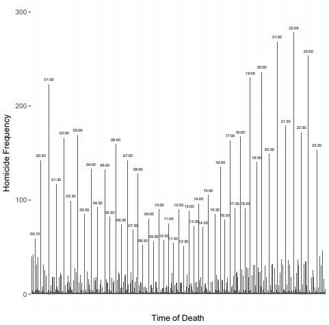
In the descriptive analysis of the days of the week, it was observed that there
is, significantly,7 a greater concentration of homicides on weekends (Saturday and
Sunday), while the days that showed a lower degree of occurrence are midweek
days such as Tuesday or Wednesday. The distribution of homicides on weekdays is
well defined having high values on weekends followed by a gradual reduction to
mid-week and then a gradual rise to arrive at the weekend again. Therefore, there
is a “day-of-the-week” effect that must be included in the analysis.
 This result can be observed in Andresen (2014) who describes the importan-
ce of criminological day in which the temporally referenced crime data is organized
along a timeline having the days of the week as reference. Although we do not find
a formal theory that describes the reasons for the greater occurrence of crimes at
the end of the week, there are countless studies that show the highest occurrence
of the crimes at the weekend such as Ceccato (2005), Ceccato and Uittenboga-
ard (2014), Andresen and Malleson (2015), Michel et al. (2016), Newton and Hirs-
chfield (2009), suggesting the existence of a possible weekend effect. The mecha-
nism of transmission is not clear, but according to these studies, this effect would be
related to the increase of agglomerations and the use of alcohol at the weekends.
 Regarding the death schedules, the distribution is quite interesting and Figure
4.3 shows the frequency of homicides that were recorded for every minute of the
day of the entire study sample.8 In this frequency chart, it is highlighted with labels
the times that presented values above 50 and it is possible to analyze that, except
for the time of the first ten minutes of the morning, they are all well-defined hours
of the day, that is, are either complete hours or half an hour. With regard to the
complete hours, stand out night schedules like 1am, 7pm, 8pm, 9pm, 10pm and
11pm. This type of behavior is in line with what was discussed in Section 1, where
an environment with poor clarity leads to delinquent behavior. This graph, there-
fore, corroborates the motivation of this paper.
 In general, it is possible to note that the overall distribution tendency of homicide
cases follows a smooth curve having a “valley” at hours close to noon and having two
“hills”. The first “hill” is represented by the hours of dawn having a peak in 1am, while
the second “hill” is located in the hours of the end of the day having its peak at 22pm.
 The complete hours have a high frequency and prominence in the graph.
However, it is also possible to observe that, interspersed with complete hours, the-
re are intermediate times appearing every half hour with a frequency pattern simi-
lar to full hours, where their highest values are at 8:30 p.m., 9:30 p.m., 10:30 p.m.

7 Kruskal-Wallis nonparametric tests were performed with Dunn’s multiple comparisons with = 5% to
 compare months of the year and days of the week. This test is analogous to Analysis of Variance (ANOVA)
 and was used because the residuals did not adhere to the normality hypothesis.
8 Part of the sample (almost 0.3%) was considered missing, since the death time field was not filled.
 In addition, we did not consider the deaths that presented the 00:00 time, placing them as missing
 as well.

18 Análise Econômica, Porto Alegre, v. 39, n. 79, p. 7-33, jun. 2021.

and 11:30 p.m. This location pattern of most criminal occurrence draws attention
to the fact that there might be a possible imprecision and knowledge of the exact
time the murder occurred. It is reasonable to assume that the real distribution is
somewhat smoother between minutes, but because of the ease and convenience
of recording, more defined times are chosen for specific hours or half an hour be-
tween these times. Despite these caveats with respect to the data it is possible to
visualize more “broken” times illustrated in small bars along the graph of Figure 4.

Figure 4 – Homicide rates by time of occurrence in Rio Grande do Sul

Source: SIM ([2018]); FEE ([2018]).

 Through the INMET data it is possible to analyze if there is some kind of rela-
tion between criminal rates and climatic variables. The main variable that proved
to be important in the homicidal relationship was the average temperature of the
days. There is a trend that on warmer days, homicidal rates are higher. Most linear
correlations were positive and significant ( = 5%).
 The relation of temperature to criminal behavior has already been discus-
sed in some studies in the literature. Ranson (2014) shows that, for US, there is a
strong positive effect between monthly temperature and murder, rape, theft, vehi-
cle theft, among others. Gamble and Hess (2012) verify that, for Dallas, the daily
temperature had a strong relation with severe aggressions, being characterized by
an inverted U with inflection point at 32.2C. In addition, the authors found a simi-
lar relationship for sexual assaults and homicides, but not very explanatory. Britto
(2014) analyzes criminal data from Juiz de Fora (Brazilian state of Minas Gerais)

 Análise Econômica, Porto Alegre, v. 39, n. 79, p. 7-33, jun. 2021. 19

and several climatic variables, where the monthly temperature is related to death
by homicide. For Pelotas (Brazilian city of Rio Grande do Sul state), Silveira and
Vieira (2001) analyze graphically the positive relation between the increase of the
monthly temperature and the increase of the homicides.

4.2 Regression Discontinuity: Start of DST

 In this section we present the main results of the estimated RDDs for the DST
entry period. The main models follow the structure similar to that described in Sec-
tion 3.2, being represented by two equations: one adding covariates and other not.
Equation 7 represents the complete model:

 = 0 + ( ≥ 0) + ( ) + 1 mp + 2 r + 3 ind + k y + a (7)

 Where = , , ..., the index of the day-of-week fixed
effect (sunday is the reference category), o index of the day and the year index,
where each equation is estimated for each year separately. The dependent variable
is (homicide rate) and the covariates are abbreviated as emp (temperature),
 r (pluviometric precipitation) and in (wind speed). In addition, we estimate
a model without covariates, according to Equation 8:
 = 0 + ( ≥ 0) + ( ) + . (8)

 Regarding DST entry, the main results are summarized in Table 3 and Figure 5.9
In all years and models it was observed a high absence of significance with the excep-
tion for the model with no covariates in 2007 that showed some level of significance
below = 0.05. The results of the discontinuity effect indicate that, for DST entry, there
is neither increase nor drop in homicide rates indicating that, if any, it is due only to ran-
dom fluctuations of the data. Only in 2007, there is an indication of the positive effect
of DST on criminal rates of = 0.0195, i.e., with an opposite direction than expected.
 Figure 5 illustrates the main results of the nonparametric regressions betwe-
en the period prior to the implementation of the DST (Pre-Period) and the later
period (Post-Period) for the models without covariates. It is possible to verify that
the local regression curves do not, in fact, show any signs of abrupt changes of
direction when it crosses = 0. In addition, the 95% confidence intervals between
pre- and post-discontinuity period have a large intersection in values. In this figure,
however, we can note the result consistent with the only significance found in the

9 It makes sense to take a look, previously, at the effect of possible discontinuity on covariates to
 justify their use in increasing the precision of . According to them, we can see that there is little
 (or no) significant discontinuity effect of the DST entry in climate variables, except for a drop in
 temperature in 2006 (Sig. ≈ 0.0266), an increase in precipitation in 2006 (Sig. ≈ 0.0243), a fall in
 precipitation in 2014 (Sig. ≈ 0.0259) and an increase in wind speed in 2013 (Sig. < 0.0001).

20 Análise Econômica, Porto Alegre, v. 39, n. 79, p. 7-33, jun. 2021.

previous Table 3 for the year 2007. In the central upper chart, the nonparametric
trend of the post intervention period goes up when = 0 indicating an increase in
the homicide rate soon after DST entry.

Table 3 – Local effects of DST entry for all years and models
 Year Effects ( ) Significance Does it include covariates?
 2006 0.0116 0.1431 Yes
 2006 0.0134 0.1807 No
 2007 0.0175 0.0600 Yes
 2007 0.0195 0.0300 No
 2008 0.0046 0.6345 Yes
 2008 0.0060 0.5807 No
 2009 -0.0043 0.6054 Yes
 2009 -0.0034 0.6827 No
 2010 -0.0077 0.3085 Yes
 2010 -0.0029 0.6966 No
 2011 0.0000 0.9991 Yes
 2011 0.0012 0.8814 No
 2012 -0.0084 0.3536 Yes
 2012 -0.0090 0.3524 No
 2013 -0.0010 0.9171 Yes
 2013 -0.0004 0.9638 No
 2014 0.0041 0.6898 Yes
 2014 0.0095 0.4035 No

Source: Elaborated by the author.

Figure 5 – Regression discontinuity at the entrance of DST in models without covariables.

Source: Elaborated by the author; SIM ([2018]); FEE ([2018]).

 Análise Econômica, Porto Alegre, v. 39, n. 79, p. 7-33, jun. 2021. 21

Another interesting result to analyze is the relation of the climatic covariates
in the regressions of the Model 1. We assess the effect of all the years of temperatu-
re, precipitation and wind speed. Again, most of the effects are null, except for the
average temperature that, in 2006, 2013 and 2014, was positively related to homi-
cide rates. In addition, in 2008, there was an inverse effect between wind speed
and rate, indicating that this year, as there was more wind in RS, there were fewer
homicides (Sig. = 0.0408).
 The weekday covariates were the ones that presented the most relevant in
the model as previously discussed. The weekday effect is negative and significant in
most of the betas, indicating a Sunday homicide.
 A very important feature of the intervention, which cannot be ignored, is that
both the start and the end of DST, always occur at dawn between Saturday and
Sunday. Moreover, we found that the day of the week has a considerable influence
on criminal practice both in descriptive terms, as seen in Section 4.1, and in infe-
rential terms as now analyzed in the effect of its covariate. However, the effect of
Saturday in relation to Sunday (illustrated by the coefficient of Saturday) is not so
strong and, for the most part, it is not significant what indicates that there is a “we-
ekend effect” in criminal activity. That is, there is a historical “weekend” disconti-
nuity while DST will necessarily be confused with the “Saturday vs. Sunday” effect.
Since the effect of the discontinuity of the regression is local and takes into account
the neighborhood of the points the effect, “Friday vs. Saturday” locally affects the
transition “Saturday vs. Sunday”.

4.3 Regression Discontinuity: End of DST

 In this section we present the results of DST ending.10 Table 4 and Figure 6
illustrate the main results of this approach.

Table 4 – Local effects of DST ending for all years and models
 Year Effects ( ) Significance Does it include covariates?
 2006 -0.0039 0.6746 Yes
 2006 0.0051 0.6176 No
 2007 0.0129 0.1983 Yes
 2007 0.0096 0.3610 No
 2008 -0.0132 0.1825 Yes
 Continua...

10 Previously, it makes sense to analyze the discontinuity effect on covariates. In most of the models,
 there was no significance, but in other years these discontinuities deserve attention. In relation to
 temperature, we can see that in general there is a decreasing trend of temperature as leaving the
 summer. However, we see positive discontinuities with effect of 2.59 in 2007 (Sig. = 0.0033) and
 1.54 in 2009 (Sig. = 0.0292). Regarding precipitation, we noticed a discontinuity of 5.42 in 2006
 (Sig. = 0.0254) and -11.64 in 2007 (Sig. < 0,001). The wind speed presented discontinuity in 2006
 (0,53 with Sig. = 0.0375), 2009 (-0,499 with Sig. = 0.0355) and 2013 (0,7565 with Sig. = 0.0154).

22 Análise Econômica, Porto Alegre, v. 39, n. 79, p. 7-33, jun. 2021.

Conclusão.

 Year Effects ( ) Significance Does it include covariates?
 2008 -0.0070 0.4690 No
 2009 -0.0143 0.0880 Yes
 2009 -0.0088 0.3622 No
 2010 -0.0130 0.2104 Yes
 2010 -0.0125 0.1933 No
 2011 0.0058 0.4814 Yes
 2011 0.0077 0.3804 No
 2012 0.0073 0.3544 Yes
 2012 0.0091 0.3198 No
 2013 -0.0374 0.0002 Yes
 2013 -0.0346 0.0007 No
 2014 0.0092 0.4569 Yes
 2014 0.0057 0.6194 No

Source: Elaborated by the author.

Figure 6 – Regression discontinuity at the end of DST in models without covariates

Source: Elaborated by the author; SIM ([2018]); FEE ([2018])..

 Análise Econômica, Porto Alegre, v. 39, n. 79, p. 7-33, jun. 2021. 23

There is absence again of statistical significance in all the years of the series.
Virtually all effects estimated for do not have any statistical evidence indicating
discontinuity, with the exception of the year 2013. This year we saw that we had the
negative effect of = 0.0374 for the model with covariates and = 0.0346 for the
simplest model. What draws attention, again, to this result is that the direction of the
effect is the opposite of what is expected. The intervention of leaving the DST implies
less light during the day which would lead to an increase in the homicide rate, which
was not the case. In addition, it should be considered that, in this year there was an
abrupt increase in wind speed just at the exit of the DST. Therefore, this effect of re-
ducing crime may be confused with increasing wind speed, since we have seen that
these two variables can be related according to the already discussed results.
 With regard, the effect of the covariates on the end of DST, only Temperature
in 2012 ( = 0.0021 e Sig. = 0.0149) and Wind Speed in 2006 ( = 0.0096 e Sig.
= 0.0313) showed significant results. Again, there is evidence that as temperatures
rise, criminal rates increase as well. On the other hand, the Wind Speed result indi-
cates that, in 2006, as there is more wind, higher homicide rates occur.
 The effects of the weekdays at the exit of DST and their indications are ana-
logous to those discussed in Section 4.2. It is possible to note that the “weekend”
effect remains present since Saturday’s ’s are not significant and weekdays have
significant negative effect for most of the values.
 In general, these results of the end of DST only confirm the main results found
for the start period. That is, without evidence that DST has an influence on crime.
In terms of model results with covariables, it was observed that in both cases, we-
ekend effects are strong and there is evidence of a positive relationship between
temperature and homicide in some years (especially in start models for DST).

5 Robustness Checks

 The results found do not indicate a significant effect in many of the cases of
DST in homicide rates. This section is devoted to evaluating the method used un-
der different estimation techniques.

5.1 Estimation with Demean Approach

 The first robustness check is given by the nature of the variable to be esti-
mated in the discontinuity regression. The demean method used in Smith (2016)
and Toro et al. (2016) seeks to remove the possible confounding effects of the me-
thod by correcting the dependent variable by making the logarithm of the value
adjusted by the mean of homicides occurred on that day of the week, in that speci-

24 Análise Econômica, Porto Alegre, v. 39, n. 79, p. 7-33, jun. 2021.

fic region and in that specific year.11 In this case, there would be no need to inclu-
de weekday covariates nor the need to estimate separate models per year, but it
would make the use of climatic covariates unfeasible. In this sense, the model to be
estimated follows the Equation 8. In both results, we again verified the non-signifi-
cance of the DST effect for both start and end models. This result is in line with the
findings of this study, indicating that there is no effect of DST on homicides in RS.

5.2 Sex Difference

 The possible sudden change in homicide rates that the DST might cause
could have could affect differently depending on the sex of the victim.12 Although
the sex differences in crime has already been studied in the literature (ROWE et
al., 1995; FOX; FRIDEL, 2017), it is unheard in the literature the difference in the
effects related to the implementation DST policy. It was conducted nonparametric
differences-in-differences (diff-in-diff) according to Equation 9 for the demean ap-
probeginningthe beggining and the end of DST period.

 = 0 + ( s ≥ 0) + ( s) + ( s ≥ 0) × ( s) + ( s) + s (9)

 In this model, assuming similar tendencies close to the change in the DST
for men and women, it captures this sex effect through the τE which evaluates the
difference of sex in the differences of periods. For more details of the diff-in-diff ap-
proach we recommend Angrist and Pischke (2013).
 Both models were estimate and the results point the absence of differences
in sex for either entry or end of DST. For the initial model was estimated in -0.02
with significance of 0.77 and, for the model of the end of DST, the same parameter
was estimated in -0.09 with significance of 0.21. Therefore, the absence of signifi-
cance evaluated that there is no evidence that the DST affects differently men and
women in the dataset.

5.3 Bandwidth Choice

 One of the components of nonparametric estimation is the choice of the
smoothing parameter (or bandwidth) in the local regression. Calonico et al. (2014)
discuss robust ways of estimating discontinuity regressions, as well as proposing

11 This method adjusts the number of homicides on each day of the week in each region in each year by
 the average number of homicides occurred on that day of the week, in that region and in that speci-
 fic year. For example, the dependent variable for, to say, the Monday following the DST transition in
 the state of RS in the year of 2008 is the logarithm of the number of homicides on that Monday in RS
 divided by the average number of homicides occurred during all the Mondays of 2008 in RS.
12 We thank the reviewer for pointing out the possibility of this robustness check.

 Análise Econômica, Porto Alegre, v. 39, n. 79, p. 7-33, jun. 2021. 25

alternative bandwidths. Using the authors’ approach, we estimated the start and
end models of DST.13
 Table 5 shows the results of the effect of DST ( ) on start and end models.
Although there was a larger set of significance, the changes were not very substan-
tial since, again, in virtually all models and years there was no significant effect of
 . The biggest highlights of the entry are in 2006, 2010 and 2013 for models with
covariates. Regarding the end of DST, this bandwidth pointed out some interesting
significance as an increase in the homicide rate in 2007 in both models and a re-
duction in the rate in 2013 in line with the results previously presented.

Table 5 – Results of DST using alternative bandwidth
 Does it include Does it include
 Effects ( ) Significance Effects ( ) Significance
 Year covariates? covariates?
 Entry End
 2006 0.0404 0.0001 Yes 0.0690 0.0097 Yes
 2006 0.0242 0.3121 No 0.0192 0.2072 No
 2007 0.0088 0.5503 Yes 0.0545 0.0000 Yes
 2007 0.0287 0.0764 No 0.0332 0.0006 No
 2008 0.0125 0.0563 Yes -0.1228 0.0000 Yes
 2008 0.0254 0.3210 No -0.0463 0.2834 No
 2009 -0.0112 0.2031 Yes 0.0134 0.3403 Yes
 2009 0.0062 0.8225 No 0.0133 0.6456 No
 2010 -0.0145 0.0273 Yes -0.0234 0.0001 Yes
 2010 0.0012 0.9505 No -0.0131 0.3561 No
 2011 -0.0033 0.6611 Yes 0.0029 0.6365 Yes
 2011 -0.0017 0.9028 No -0.0101 0.5902 No
 2012 0.0044 0.5971 Yes -0.0040 0.6762 Yes
 2012 -0.0046 0.7194 No 0.0255 0.0867 No
 2013 0.0187 0.0004 Yes -0.0264 0.0104 Yes
 2013 0.0130 0.3171 No -0.0404 0.0507 No
 2014 0.0172 0.0730 Yes -0.0059 0.4047 Yes
 2014 -0.0042 0.8693 No 0.0057 0.6762 No

Source: Elaborated by the author.

13 We highlight that, for this, it was necessary to make use of the rdrobust package presented and des-
 cribed in Calonico et al. (2015) in software R (R CORE TEAM, 2016), where the optimal bandwidth
 used in this section minimizes the mean squared error. In Section 4, the estimation was performed
 using Generalized Additives Models and the package gam (HASTIE, 2017) was used because with
 it the marginal effects of covariates could be analyzed.

26 Análise Econômica, Porto Alegre, v. 39, n. 79, p. 7-33, jun. 2021.

5.4 Most affected Hours by the DST

 One of the main hypotheses raised in Doleac and Sanders (2005) and Toro et
al. (2016) is that DST has a more pronounced effect in the hours closer to the tran-
sition between day and night, that is, in the hours closer to sunset. In these works,
there is evidence that the effects are greater at times close to sunset. In this sense, it
is also of interest to verify if this hypothesis holds for the case of RS.14
 We investigated the results of the entry and exit, respectively, of the DST by
the demean method making use of only the cases that happened near the sunset. In
the period of entry, again, we see no significant effect on the transition. However, in
the case of exit we observed weak but non-significant (Sig. = 0.0668) evidence that
there was an increase in homicide rate, which is in the sense of the main hypothesis
of this article that less light indicates an increase in delinquency practice.

5.5 Analysis at All Death Occurrence Location

 In Section 3.1, it is described that the models are estimated only in cases whe-
re the death occurred outside hospitals and other health facilities implying a loss of
27.54% of cases. Such treatment is due to the fact that it is possible that there is a
reallocation of the day between the criminal occurrence and the time of death, so-
mething that is undesirable in this article considering the character of daily analysis
of the local effect of DST. However, it is possible to assume that this loss of sample
will affect the estimated results of this paper.
 In this sense, this Section 5.5 is dedicated to presenting the results taking into
account the whole universe of homicides of the base of the SIM independent of
the place of criminal occurrence. It is noteworthy that between 2006 and 2014 this
entire base results in 19,318 cases.
 Table 6 shows the local effects of DST taking into account all cases of the
database regardless of the place of occurrence. For the start models in the DST,
again we did not identify any substantial changes in relation to the absence of
significance of the Table 4.1, except that with this approach the year of 2010 (with
covariates) showed a significant reduction and not in the year of 2007 (without
covariates) as seen previously. Regarding the end of the DST, the consonance with
the results obtained is even greater, because, again, only the year of 2013 had a
significant reduction in the models in the same way as was discussed in Section 4.3.

14 The time considered as close to sunset is between 17pm and 21pm.

 Análise Econômica, Porto Alegre, v. 39, n. 79, p. 7-33, jun. 2021. 27

Table 6 – Local effects of the DST for all years and models: all occurrence locations
 Does it include Does it include
 Effects ( ) Significance Effects ( ) Significance
 Year covariates? covariates?
 Entry End
 2006 0.0041 0.6962 Yes 0.0007 0.9465 Sim
 2006 0.0053 0.6621 No 0.0071 0.5742 Não
 2007 0.0036 0.7122 Yes 0.0120 0.2709 Sim
 2007 0.0061 0.5361 No 0.0121 0.3227 Não
 2008 -0.0034 0.7700 Yes -0.0192 0.0901 Yes
 2008 0.0020 0.8825 No -0.0137 0.2676 No
 2009 -0.0070 0.4778 Yes 0.0003 0.9765 Yes
 2009 -0.0026 0.7923 No 0.0053 0.6663 No
 2010 -0.0221 0.0134 Yes -0.0176 0.2050 Yes
 2010 -0.0147 0.1198 No -0.0176 0.1851 No
 2011 0.0016 0.8427 Yes -0.0010 0.9155 Yes
 2011 0.0034 0.6857 No 0.0011 0.9102 No
 2012 -0.0014 0.8846 Yes -0.0097 0.2710 Yes
 2012 -0.0007 0.9471 No -0.0068 0.4835 No
 2013 -0.0029 0.7828 Yes -0.0406 0.0008 Yes
 2013 -0.0020 0.8539 No -0.0341 0.0052 No
 2014 0.0018 0.8759 Yes 0.0153 0.2643 Yes
 2014 0.0072 0.5599 No 0.0119 0.3832 No

Source: Elaborated by the author.

6 Final Considerations

 The purpose of this article was to study the effect of the entry and exit of DST
on homicides in the Brazilian state of Rio Grande do Sul. The idea was to verify if
the increase of the luminosity, caused by the entrance in the DST, has deterrent
effect criminal. There is strong evidence in this sense that most homicides occur
under darkness, peaking at 10 o’clock persisting until early morning hours, indica-
ting that aggressors prefer to act during the nighttime period.
 Using the Brazilian Mortality Information System (SIM) homicide data, whi-
ch has date and time information of the event, this study evaluated the effect of
a possible discontinuity in the criminal activity both at the beginning and end of
DST in the period 2006-2014. Under the hypothesis of lightening deterrence, it was
expected that at the beginning of DST, there would be a drop in the homicide rate
and, at the end of it, an increase.
 The approach used RDD in which non-parametric models are estimated for
the pre and post-intervention period and assess whether the local effect of transi-
tion from DST intervention is significant. In addition, the idiosyncrasies of the data
are contemplated as the inclusion of fixed effect of day of the week, climatological
covariables and separate estimations per year of each model.

28 Análise Econômica, Porto Alegre, v. 39, n. 79, p. 7-33, jun. 2021.

The results showed that DST, in general, has no effect on the homicide rate.
It was evidenced that in almost all the years of the historical series the effect of the
DST was null with regard to the change in the level of the homicide rate. Besides,
in some cases the results that were significant pointed in the opposite-to-expected
sense, such as in 2007 that there was an increase in homicides when DST was star-
ted and in 2013 that there was a reduction in homicides when the DST ended.15
In this sense, although there is strong evidence that there is a luminosity effect on
criminal activity when we analyze the hours of the day the homicides occur, it is
not captured by the model when we analyze the effect of DST alone. One of the
hypotheses to be considered for this lack of effect is that, although the change in
DST time is sudden, the presence of “more” light during the day is actually gradual
and in interstices, which mitigates the sharp effect of the discontinuous interven-
tion. It is important to note that many variables affect delinquency behavior.
 History of behavioral problems in childhood (MURRAY et al., 2015), use of
alcohol (MCBRIDE et al., 1991; DEARDEN; PAYNE, 2009) and social inequality
(KELLY, 2000; FAJNZYLBER et al., 2002), for example, are factors that can influen-
ce criminal activity. Specifically, it is of interest to carry out future studies regar-
ding the relationship between alcohol consumption and homicides for RS. In the
analyzes presented here, we find that weekday plays a crucial role in criminal rates,
where the weekend is when more crimes happen. In addition, strong evidence of a
positive correlation between temperature and homicides was estimated.
 The results estimated in this article were robust to variations of model specifi-
cations. Alternative approaches were tested such as the use of the demean method
for estimation of RDD, alternative smoothing parameters, estimation for only those
cases that occurred at hours more affected by DST and not excluding occurrences
in hospitals and health facilities. In almost all situations, this intervention did not
have a good explanatory power in the change of homicide rates.
 This article advances considerably in the literature on the economics of crime
because of its pioneering character of local evaluation of the DST effect on RS
crimes. Up to the present time, no work is known that addressed this topic in the
state. The discussion of the effects of DST is extremely relevant because it is a public
policy that affects all the inhabitants of a certain place and studies that evaluate
its true impact on the most different aspects are important to subsidize the public
authorities to think/rethink this measure and its consequences in society. In 2017,
the Brazilian federal government studied the possibility of excluding DST from the
national calendar claiming that its main purpose of energy saving is not achieved,
considering also to carry out popular consultation to evaluate its revocation. In this
sense, studies like this one carried out are justified.

15 Possible confounding effect with wind speed.

 Análise Econômica, Porto Alegre, v. 39, n. 79, p. 7-33, jun. 2021. 29

References
ANDRESEN, M. A. Environmental criminology: evolution, theory, and practice. Abingdon:
Routledge, 2014.

ANDRESEN, M. A.; MALLESON, N. Intra-week spatial-temporal patterns of crime. Crime
Science, v. 4, n. 1, p. 12, 2015.

ANGRIST, J. D.; PISCHKE, J. S. Mostly harmless econometrics: an empiricist’s companion.
Princeton: Princeton University Press, 2013.

ARIES, M. B. C.; GUY, R. N. Effect of daylight saving time on lighting energy use: a literature
review. Energy Policy, v. 36, n. 6, p. 1858-1866, 2008.

ARVATE, P.; FALSETE, F. O.; RIBEIRO, F. G.; SOUZA, A. P. Lighting and violent crimes:
evaluating the effect of an electrification policy in rural Brazil on violent crime reduction.
Textos para Discussão FGV, n. 408, 2015.

BECKER, G. Crime and punishment: an economic approach. Journal of Political Economy, v.
76, n. 2, p. 169-217, 1968.

BRITTO, M. C. Análise dos homicídios ocorridos em Juiz de Fora entre os anos de 1980
a 2012 e sua relação com as condições climáticas. Revista Brasileira de Climatologia, v. 13,
2014.

CALONICO, S.; CATTANEO, M. D.; TITIUNIK, R. Robust nonparametric confidence intervals
for regression-discontinuity designs. Econometrica, v. 82, n. 6, p. 2295-2326, 2014.

CALONICO, S.; CATTANEO, M. D.; TITIUNIK, R. Rdrobust: an R package for robust non-
parametric inference in regression-discontinuity designs. R Journal, v. 7, n. 1, p. 38-51, 2015.

CECCATO, V. Homicide in São Paulo, Brazil: assessing spatial-temporal and weather varia-
tions. Journal of Environmental Psychology, v. 25, n. 3, p. 307-321, 2005.

CECCATO, V.; UITTENBOGAARD, A. C. Space-timeerseysid oerseye in stockholm, sweden.
In: SPATIAL STATISTICS–MAPPING GLOBAL CHANGE, 1., 2011, The Netherlands. Proceed-
ings […]. The Netherlands: Elsevier, 2011. p. 1-8.

CECCATO, V.; UITTENBOGAARD, A. C. Space–time dynamics of crime in transport nodes.
Annals of the Association of American Geographers, v. 104, n. 1, p. 131-150, 2014.

CLEVELAND, W. S.; DEVLIN, S. J. Locally weighted regression: an approach to regression
analysis by local fitting. Journal of the American Statistical Association, v. 83, n. 403, p. 596-
610, 1988.

COHN, E. G.; ROTTON, J. Weather, seasonal trends aerseyside crimes in minneapolis, 1987–
1988. A moderator-variable time-series analysis of routine activities. Journal of Environmental
Psychology, v. 20, n. 3, p. 257-272, 2000.

30 Análise Econômica, Porto Alegre, v. 39, n. 79, p. 7-33, jun. 2021.

DEARDEN, J.; PAYNE, J. Alcohol and homicide in Australia. Trends & Issues in Crime and
Criminal Justice, n. 372, 2009.

DEE, T.; WYCKOFF, J. Incentives, selection and teacher performance: evidence from IM-
PACT. NBER Working Paper, n. 19529, 2013.

DE SOUZA, M. F. M.; MACINKO, J.; ALENCAR, A. P.; MORAIS NETO, O. L. Reductions in
firearm-related mortality and hospitalizations in Brazil after gun control. Heath Affairs, v. 26,
n. 2, 2007.

DOLEAC, J. L.; SANDERS, N. J. Under the cover of darkness: how ambient light influences
criminal activity. Review of Economics and Statistics, v. 97, n. 5, p. 1093-1103, 2005.

FAJNZYLBER, P.; LEDERMAN, D.; LOAYZA, N. Inequality and violent crime.

The Journal of Law and Economics, v. 45, n. 1, p. 1-39, 2002.

FARRELL, G.; PEASE, P. Crim seasonality: domestic disputes and residential burglary in Mer-
seyside 1988-90. The British Journal of Criminology, v. 34, n. 4, p. 487-498, 1994.

FUNDAÇÃO DE ECONOMIA E ESTATÍSTICA (FEE). Available at: https://arquivofee.rs.gov.
br/. Access: Apr. 10, 2021.

FIELD, S. The effect of temperature on crime. The British Journal of Criminology, v. 32, n. 3,
p. 340-351, 1992.

FOX, J. A.; FRIDEL, E. E. Gender differences in patterns and trends in US homicide, 1976–
2015. Violence and Gender, v. 4, n. 2, p. 37-43, 2017.

GAMBLE, J. L.; HESS, J. J. Temperature and violent crime in Dallas, Texas: relationships and
implications of climate change. Western Journal of Emergency Medicine, v. 13, n. 3, p. 239,
2012.

HASTIE, T. GAM: generalized additive models. R package version 1.14- 4. [S. l.]: Stanford Uni-
versity, 2017. Available at: https://CRAN.R-project.org/package=gam. Access: Jan. 19, 2021.

HORROCKS, J.; MENCLOVA, A. K. The effects of weather on crime. New Zealand Economic
Papers, v. 45, n. 3, p. 231-254, 2011.

KELLOGG, R.; WOLFF, H. Daylight time and energy: evidence from an Australian experi-
ment. Journal of Environmental Economics and Management, v. 56, n. 3, p. 207-220, 2008.

KELLY, M. Inequality and crime. The Review of Economics and Statistics, v. 82, n. 4, p. 530-539,
2000.

KOTCHEN, M. J.; GRANT, L. E. Does daylight saving time save energy? Evidence from a natural
experiment in Indiana. The Review of Economics and Statistics, v. 93, n. 4, p. 1172-1185, 2011.

KOUNTOURIS, Y.; REMONDOU, K. About time: daylight saving time transition and indi-
vidual well-being. Economics Letters, v. 122, n. 1, p. 100-103, 2014.

 Análise Econômica, Porto Alegre, v. 39, n. 79, p. 7-33, jun. 2021. 31