DEEP LEARNING FOR VEHICLE DETECTION IN AERIAL IMAGES - tnt.uni ...
←
→
Page content transcription
If your browser does not render page correctly, please read the page content below
DEEP LEARNING FOR VEHICLE DETECTION IN AERIAL IMAGES

                     Michael Ying Yang                                          Wentong Liao, Xinbo Li, Bodo Rosenhahn

              Scene Understanding Group                                              Institute for Information Processing
                 University of Twente                                                   Leibniz University Hannover

                             ABSTRACT                                             search. It’s low efficient and leads to costly and redundant
                                                                                  computation. The window’s sizes and sliding steps must be
The detection of vehicles in aerial images is widely applied in
                                                                                  carefully chosen to adapt the varieties of objects of interest in
many domains. In this paper, we propose a novel double focal
                                                                                  dataset.
loss convolutional neural network framework (DFL-CNN). In
the proposed framework, the skip connection is used in the
CNN structure to enhance the feature learning. Also, the fo-
cal loss function is used to substitute for conventional cross
entropy loss function in both of the region proposed network
and the final classifier. We further introduce the first large-
scale vehicle detection dataset ITCVD with ground truth an-
notations for all the vehicles in the scene. The experimental
results show that our DFL-CNN outperforms the baselines on
vehicle detection.
   Index Terms— Vehicle detection, convolutional neural
network, focal loss, ITCVD dataset
                                                                                    Fig. 1. Vehicles detection results on the proposed dataset.
                       1. INTRODUCTION
                                                                                      In recent years, deep convolutional neural network (DCNN)
The detection of vehicles in aerial images is widely applied in                   has achieved great successes in different tasks, especially for
many domains, e.g.traffic monitoring, vehicle tracking for se-                    object detection and classification [8, 9]. In particular, the se-
curity purpose, parking lot analysis and planning, etc. There-                    ries of methods based on region convolutional neural network
fore, this topic has caught increasing attention in both aca-                     (R-CNN) [10, 11, 12] push forward the progress of object de-
demic and industrial fields [1, 2, 3]. However, compared with                     tection significantly. Especially, Faster-RCNN [12] proposes
object detection in ground view images, vehicle detection in                      the region proposal network (RPN) to localize possible ob-
aerial images has a lot of different challenges, such as much                     ject instead of traditional sliding window search methods and
smaller scale, complex backgrounds and the monotonic ap-                          achieves the state-of-the-art performance in different datasets
pearance. See Figure 1 for an illustration.                                       in terms of accuracy. However, these existing state-of-the-
    Before the emergence of deep learning, hand-crafted                           art detectors cannot be directly applied to detect vehicles in
features combined with a classifier are the mostly adopted                        aerial images, due to the different characteristics of ground
ideas to detect vehicles in aerial images [4, 1, 2]. However,                     view images and aerial view images [13]. The appearance of
the hand-crafted features lack generalization ability, and the                    the vehicles are monotone, as shown in Figure 1. It’s diffi-
adopted classifiers need to be modified to adapt the of the                       cult to learn and extract representative features to distinguish
features. Some previous works also attempted to use shal-                         them from other objects. Particularly, in the dense park lot, it
low neural network [5] to learn the features specifically for                     is hard to separate individual vehicles. Moreover, the back-
vehicle detection in aerial images [6, 7]. However, the rep-                      ground in the aerial images are much more complex than the
resentational power of the extracted features are insufficient                    nature scene images. For examples, the windows on the fa-
and the performance meets the bottleneck. Furthermore, all of                     cades or the special structures on the roof, these background
these methods localize vehicle candidates by sliding window                       objects confuse the detectors and classifiers.Furthermore,
                                                                                  compared to the vehicle sizes in ground view images, the
     The work is funded by DFG (German Research Foundation) YA 351/2-1
and RO 4804/2-1. The authors gratefully acknowledge NVIDIA Corporation
                                                                                  vehicles in the aerial images are much smaller (ca. 50 × 50
for the donated GPU used in this research. We thank Slagboom en Peeters           pixels) while the images have very high resolution (normally
for providing the aerial images. Contact email: michael.yang@utwente.nl           larger than 5000 × 2000 pixels). Lastly, large-scale and well

978-1-4799-7061-2/18/$31.00 ©2018 IEEE                                      3079                                                                  ICIP 2018

Authorized licensed use limited to: Technische Informationsbibliothek (TIB). Downloaded on April 14,2021 at 15:06:05 UTC from IEEE Xplore. Restrictions apply.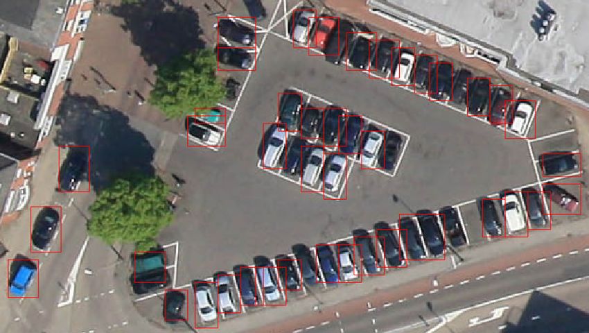
annotated dataset is required to train a well performed DCNN 2.1. Skip Connection
methods. However, there is no public large-scale dataset,
It has been proven in the task of semantic segmentation that,
such as ImageNet [14], for vehicle detection in aerial im-
features from the shallower layers retain more detail informa-
ages. The two exceptions are VEDAI dataset [15] and DLR
tion [19]. In the task of object detection, the sizes of vehicles
3K dataset [2]. However, the objects in the VEDAI dataset
in aerial images are ca. 30 × 50 pixels, assuming 10cm GSD.
are relative easy to detect because of the small number of
The size of the output feature maps of the ResNet from the
vehicles which sparsely distribute in the images, and the
5th pooling layers is only one 32nd of the input size [17].
background is simple. The more challenging and realistic
The shorter edges of most vehicles are very small when they
DLR 3K dataset contains totally 20 aerial images with reso-
are projected on the feature maps after the 5th pooling layer.
lution of 5616 × 3744. 10 images (3505 vehicles) are used for
So, they will be ignored because their sizes are rounded up.
training. Such number of training samples seems too small
Furthermore, pooling operation leads to significant loss of de-
for training a CNN model.
tailed information. For densely parked area, it is difficult to
To address these problems, we propose a specific frame-
separate individual vehicles. For example, the extracted fea-
work for vehicle detection in aerial images, as shown in Fig-
tures from the shallow layer have richer detailed information
ure 2. The novel framework is called double focal loss convo-
than the features from the deeper layer. In the case of densely
lutional neural network (DFL-CNN), which consists of three
parked area, the detail information play an important to sep-
main parts: 1) A skip-connection from the low layer to the
arate the individual vehicles from each other. Therefore, we
high layer is added to learn features which contains rich detail
fuse the features from the shallow layers, which contain more
information. 2) Focal loss function [16] is adopted in the RPN
detail information, with the features learned by deeper layers,
instead of traditional cross entropy. This modification aims at
which have more representative abilities, to precisely localize
the class imbalance problem when RPN determine whether
detected individual vehicle. This skip-connected CNN archi-
a proposal is likely an object of interest. 3) Focal loss func-
tecture is illustrated in Figure 3. The image fed to the network
tion replaces the cross entropy in the classifier. It’s used to
is 752 × 674 pixels. The size of the feature maps from the 4th
handle the problem of easy positive examples and hard neg-
and 5th pooling layers are 42 × 47 × 1024 and 21 × 24 × 2048
ative examples during training. Furthermore, we introduce a
respectively. To fuse them together, the smaller feature maps
novel large-scale and well annotated dataset for quantitative
are upsampled to the size of 42 × 47 × 2048, and then re-
vehicle detection evaluation - ITCVD. Towards this goal, we
duced the feature channels into 1024 by a 1 × 1 convolution
collected 173 images with 29088 vehicles, where each vehicle
layer. Then the two feature maps are concatenated as the skip-
in the ITCVD dataset is manually annotated using a bound-
connected feature maps.
ing box. The performance of the proposed method is demon-
strated with respect to the state-of-the-art baseline. We make
Image Size
our code and dataset online available. 752 x 674 x 3
conv1
376x337x64
conv2
188x169x256
conv3 conv4 conv5 Upsampling Convolution
94x84x512 47x42x1024 24x21x2048 47x42x2048 47x42x1024
2. PROPOSED FRAMEWORK Concatenate
Skip-connected
feature map
An overview of the proposed framework is illustrated in Fig- Max pooling
ure 2. It’s modified based on the standard Faster R-CNN [12].
We refer readers to [12] for the general procedure of object
detection. In this work, we choose ResNet [17] as the back- Fig. 3. Structure of skip-connected CNN. The feature maps
bone structure for feature learning, because of its high effi- from the conv5 are upsampled to the same size as the feature
ciency, robustness and effectiveness during training [18]. maps from conv4. Then, the number of the feature channels
are reduced by 1 × 1 convolution layer into 1024. Finally, the
Input
Skip-connected CNN feature maps from conv4 and conv5 are concatenated.
RPN Detector
Conv Focal loss
for detection Focal loss
UpSa Feature vector for classifier
Bounding box
regression
conv1 conv2 conv3 conv4 conv5
ROI Pooling Layer
Regression
2.2. Focal loss function
Focal loss function is originally proposed by [16] to dedi-
Fig. 2. The overview of the proposed framework DFL-CNN. cate the class imbalance problems for the one-stage object
It consists of three main parts: 1) A skip-connection from the detectors, such as YOLO [20] and SSD [21]. As discussed
low layer to the high layer is added to learn features which in the paper, a one-stage detector suffers from the extreme
contains rich detail information. 2) Focal loss function [16] foreground-background class imbalance because of the dense
is adopted in the RPN instead of traditional cross entropy. 3) candidates which cover spatial positions, scales, and aspect
Focal loss function replaces the cross entropy in the classifier. ratios. A two-stage detector handles this challenge in the first
3080
Authorized licensed use limited to: Technische Informationsbibliothek (TIB). Downloaded on April 14,2021 at 15:06:05 UTC from IEEE Xplore. Restrictions apply.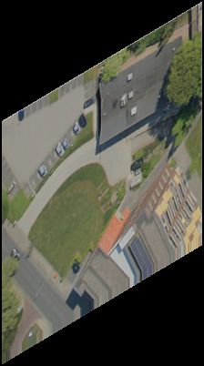
stage: candidates proposal, e.g.RPN [12], most of the candi-                      overlapping area of box of candidate and the ground truth
dates which are likely to be the background are canceled, and                     box, and the denominator represents the union of them. The
then the second stage: classifier works on much sparser can-                      proposals which have the IoU more than 0.7, are labeled as
didates. However, in the scenes with dense objects of interest,                   positive samples and the ones whose IoU are smaller than
e.g., the parking cars in Figure 1, even the state-of-the-art can-                0.1 are labeled as the negative samples. Other proposals are
didates proposal method RPN is not good enough to filter the                      discarded. All the proposals exceeding the boundary of the
dense proposals in two aspects: 1) many of the dense propos-                      image are also discarded. During training, each mini-batch
als cover two vehicles and have high overlap with the ground                      consists of 64 positive samples and 64 negative samples.
truth, which makes it hard for the proposal methods to de-                            The loss function for training the RPN using focal loss is
termine whether they are background objects. 2) Too many                          defined as:
background objects interfere the training. It is hard to select                                                  1 X
the negative samples which are very similar as the vehicles                              LRP N ({pi }, {ti }) =          Lcls−F L (pi , p∗i )
                                                                                                                Ncls i
to enhance the detector/classifier to distinguish them from the
positive samples. Inspired by the idea in [16], we proposed                                                        1 X ∗
                                                                                                              +λ          p Lreg (ti , t∗i )  (2)
to use the focal loss function instead of the conventional CE                                                    Nreg i i
loss both in the region proposal and the classification stages,
dubbed as double focal loss-CNN (DFL-CNN).                                        where Lcls−F L is the focal loss for classification, as defined
    The Focal loss is derived from the CE loss by adding a                        in Eq. (1) and Lreg is the loss for bounding box regression.
modulating factor (1 − pt )γ with tunable focusing parameter                      pi is the predicted probability of proposal i belonging to the
γ ≥ 0:                                                                            foreground and p∗i is its ground truth label. Ncls denotes the
                                                                                  total number of samples and Nreg is the total number of pos-
                LF L (pt ) = −(1 − pt )γ log(pt )              (1)
                                                                                  itive samples. λ is used to weight the loss for bounding box
The focal loss has two main properties: 1) The loss is unaf-                      regression 2 . The smooth L1 loss function is adopted for Lreg
fected by misclassified examples which have small pt when                         as in [12]. t = (tx , ty , tw , th ) is the normalized informa-
the modulating factor is near 1. In contrast, when pt → 1, the                    tion of the bounding boxes of the positive sample and t∗ is its
modulating factor is near 0 , which down-weights the loss for                     ground truth.
well-classified examples. 2)When the focusing parameter γ                             The RPN layer output a set of candidates which are likely
is increased, the effect of modulating factor is also increased.                  to be the objects of interest, i.e.vehicles in this work, and
CE is the special case of γ = 0. Intuitively, the contribution                    there predicted bounding boxes. Then, the features covered
of the easy examples are reduced while the ones from hard ex-                     by these bounding boxes are cropped out from the feature
amples are enhanced during the training. For example, with                        maps and go through the region of interest (ROI) pooling
γ = 2 1 , the focal loss of an example classified with pt = 0.9                   layer to get a fix the size of features.
is 1% of the CE loss and 0.1% of it when pt = 0.968. If an ex-                        Finally, the final classifier subnet are fed with these fea-
ample is misclassified (pt < 0.5), its importance for training                    tures and classify their labels, and predict their bounding
is increased by scaling down its loss 4 times.                                    boxes further. The loss function of the classifier subnet for
                                                                                  each candidate is formally defined as:
2.3. Double Focal Loss CNN                                                         Lclassif ier (P, T ) = Lcls−F L (P, P ∗ ) + λ2 P ∗ Lreg (T, T ∗ )
In our DFL-CNN framework, we add a skip connection to                                                                                             (3)
fuse the features from the lower (conv4) and higher (conv5)                       where T is defined as:
layers, and adopt focal loss function both in the RPN layer and                        Tx = (Px − Ax )/Aw ,               Ty = (Py − Ay )/Ah ,
the final classification layer to overcome the class imbalance
                                                                                      Tw = log(Pw /Aw ),               Th = log(Ph /Ah ),
and the easy/hard examples challenges in our task.
    As discussed in Section 2.1, the final feature maps are                            Tx∗ = (Px∗ − Ax )/Aw ,                Ty∗ = (Py∗ − Ay )/Ah ,         (4)
1/16 of the original images. Therefore, each pixel in the                             Tw∗   =   log(Pw∗ /Aw ),         Th∗   =   log(Ph∗ /Ah ),
feature maps corresponds an region of 16 × 16 pixels. To
generate candidates proposal, centered on each pixel in the                       The Px , Ax and Px∗ denote the bounding boxes of prediction
feature maps, 9 anchors in 3 different areas (302 , 502 , 702 )                   results, anchors and ground truth. The other subscripts of y, w
and 3 different ratios (1:1, 2:1 and 1:2) are generated on the                    and h are the same as x. We set λ2 = 1 to equal the influence
original input image. Every anchor is labeled as either posi-                     of classification and bounding box prediction. During train-
tive or negative sample based on the Intersection-over-Union                      ing, the classifier subnet is trained using positive and negative
(IoU) with ground truth. The IoU is formally defined as:                          samples in ratio of 1 : 3, same as the conventional training
IoU = area(Proposal∩Ground     Truth)                                             strategy [12].
          area(Proposal∪Ground Truth) , where the numerator is the
                                                                                      2 λ is set to 15 in our experiments.Because the size of final feature maps
   1γ   is set to 2 in our experiments.                                           is 47 × 42 and totally 128 anchors are chosen, therefore the ratio is ca. 15.

                                                                            3081

Authorized licensed use limited to: Technische Informationsbibliothek (TIB). Downloaded on April 14,2021 at 15:06:05 UTC from IEEE Xplore. Restrictions apply.
3. ITCVD DATASET baseline. Figure 4 depicts the relationship between recall
rate and the precision rate of DFL-CNN, Faster R-CNN and
In this section, we introduce the new large-scale, well anno- HOG+SVM algorithms with different IoU in the ITCVD
tated and challenging ITCVD dataset. The images were taken dataset. It is obvious that the CNN based methods (DFL-
from an airplane platform which flied over Enschede, The CNN in green curve and Faster R-CNN in red curve) are
Netherlands, in the height of ca 330m above the ground 3 . The significantly better than the traditional method (HOG+SVM
images are taken in both nadir view and oblique view The tilt in black curve). In the relation between recall and precision,
angle of oblique view is 45 degrees. The Ground Sampling our DFL-CNN method also perform better than Faster R-
Distance (GSD) of the nadir images is 10cm. CNN. According to these relationship curves, IoU = 0.3 is
The raw dataset contains 228 aerial images with high res- a good balance point for the following experimental settings,
olution of 5616 × 3744 pixels in JPG format. Because the which reports high recall rate and precision at the same time.
images are taken consecutively with a small time interval, Note that, it is also a conventional setting in the task of object
there is ca. 60% overlap between consecutive images. It is detection. The quantitative results of these three methods are
important to make sure that, the images used for training do given in Table 1 (the results are given with IoU = 0.3). We
not have common regions with the images that are used for can see that, our method outperforms the others.
testing. After careful manual selection and verification, 173
images are remained among which 135 images with 23543 1
0.9
DFL-CNN
Faster-RCNN
HOG+SVM
1
0.9
DFL-CNN
Faster-RCNN
HOG+SVM
0.9
0.8
DFL-CNN
Faster-RCNN
0.8 0.8
vehicles are used for training and the remaining 38 images 0.7
0.6
0.7
0.6
0.7
Precision
Precision
Recall
with 5545 vehicles for testing. Each vehicle in the dataset is 0.5
0.4
0.5
0.4
0.6
0.5
0.3 0.3
manually annotated using a bounding box which is denoted 0.2
0.1
0.2
0.1
0.4
as (x, y, w, h), where (x, y) is the coordinate of the left-up 0
0 0.1 0.2 0.3 0.4 0.5
IoU
0.6 0.7 0.8 0.9 1
0
0 0.1 0.2 0.3 0.4 0.5
IoU
0.6 0.7 0.8 0.9 1
0.3
0.8 0.85 0.9
Recall
0.95 1
corner of the box, and (w, h) is the width and height of the
box respectively. Fig. 4. The relationship between IoU and recall rate (a), IoU
and precision rate (b) and recall and precision (c) of DFL-
4. EXPERIMENTS CNN, Faster R-CNN, HOG+SVM in the ITCVD dataset.
4.1. Dataset and experimental settings
HOG+SVM Faster R-CNN DFL-CNN
We evaluate our method in our ITCVD dataset 4 . To save RR 21.19% 88.38% 89.44%
the GPU memory, each original image in the datasets are PR 6.52% 58.36% 64.61%
cropped into small patches uniformly. The resulting new im- F1-score 0.0997 0.7030 0.7502
age patches are in the size of 674×752 pixels. The coordinate
information of annotation is also updated in the new cropped Table 1. Comparison of baselines and the DFL-CNN method
patches. The deep learning models are implemented in Keras in ITCVD dataset.
with TensorFlow backend. The ResNet-50 network [17] is
used as the backbone CNN structure for feature learning for
Faster R-CNN [12] and our model. We use a learning rate of 5. CONCLUSION
0.00001 to train the RPN. The CNN structure are pre-trained
on ImageNet dataset [14]. In this paper, we have proposed a specific framework DFL-
To evaluate the experimental results, the metrics of re- CNN for vehicle detection in the aerial images. We fuse
call/precision rate and F 1-score are used, which are formally the features properties learned in the lower layer of the net-
TP
defined as: Recall Rate (RR) = TP+FN , Precision Rate (PR) = work (containing more spatial information) and the ones from
TP 2×RR×PR
TP+FP , F1-score = RR+PR , where T P , F N , F P denote the higher layer (more representative information) to enhance the
true positive, false negative and false positive respectively. network’s ability of distinguishing individual vehicles in a
Furthermore, the relationships between the IoU and RR, P R crowded scene. To address the challenges of class imbal-
are also evaluated respectively. ance and easy/hard examples, we adopt focal loss function in-
stead of the cross entropy in both of the region proposal stage
4.2. Results on ITCVD dataset and the classification stage. We have further introduced the
first large-scale vehicle detection dataset ITCVD with ground
The state-of-the-art object detector Faster R-CNN [12] is truth annotations for all the vehicles in the scene. Compared
implemented to provide a strong baseline. In addition, tra- to DLR 3K dataset, our benchmark provides much more ob-
ditional HOG + SVM method [22] is provided as a weak ject instances as well as novel challenges to the community.
3 http://www.slagboomenpeeters.com/ For future work, we will extend DFL-CNN to recognize the
4 Further experiments on DLR 3K dataset [2] can be found in the technical
vehicle types and detect the vehicle orientations.
report https://arxiv.org/abs/1801.07339.
3082
Authorized licensed use limited to: Technische Informationsbibliothek (TIB). Downloaded on April 14,2021 at 15:06:05 UTC from IEEE Xplore. Restrictions apply.6. REFERENCES [12] Shaoqing Ren, Kaiming He, Ross Girshick, and Jian
Sun, “Faster r-cnn: Towards real-time object detection
[1] Joshua Gleason, Ara V Nefian, Xavier Bouyssounousse, with region proposal networks,” in Advances in neural
Terry Fong, and George Bebis, “Vehicle detection from information processing systems, 2015, pp. 91–99.
aerial imagery,” in IEEE International Conference on
Robotics and Automation, 2011, pp. 2065–2070. [13] Guisong Xia, Xiang Bai, Jian Ding, Zhen Zhu, Serge
Belongie, Jiebo Luo, Mihai Datcu, Marcello Pelillo,
[2] Kang Liu and Gellert Mattyus, “Fast multiclass vehi- and Liangpei Zhang, “DOTA: A large-scale dataset
cle detection on aerial images,” IEEE Geoscience and for object detection in aerial images,” CoRR, vol.
Remote Sensing Letters, vol. 12, no. 9, pp. 1938–1942, abs/1711.10398, 2017.
2015.
[14] Jia Deng, Wei Dong, Richard Socher, Li-Jia Li, Kai Li,
[3] Ziyi Chen, Cheng Wang, Huan Luo, Hanyun Wang, Yip- and Li Fei-Fei, “Imagenet: A large-scale hierarchical
ing Chen, Chenglu Wen, Yongtao Yu, Liujuan Cao, and image database,” in IEEE Conference on Computer Vi-
Jonathan Li, “Vehicle detection in high-resolution aerial sion and Pattern Recognition, 2009, pp. 248–255.
images based on fast sparse representation classification
and multiorder feature,” IEEE Transactions on Intelli- [15] Sebastien Razakarivony and Frederic Jurie, “Vehicle
gent Transportation Systems, vol. 17, no. 8, pp. 2296– detection in aerial imagery: A small target detection
2309, 2016. benchmark,” Journal of Visual Communication and Im-
age Representation, vol. 34, pp. 187–203, 2016.
[4] Tao Zhao and Ram Nevatia, “Car detection in low reso-
lution aerial images,” Image and Vision Computing, vol. [16] Tsung-Yi Lin, Priya Goyal, Ross Girshick, Kaiming He,
21, no. 8, pp. 693–703, 2003. and Piotr Dollár, “Focal loss for dense object detection,”
arXiv preprint arXiv:1708.02002, 2017.
[5] Yann LeCun, Bernhard E Boser, John S Denker, Donnie
Henderson, Richard E Howard, Wayne E Hubbard, and [17] Kaiming He, Xiangyu Zhang, Shaoqing Ren, and Jian
Lawrence D Jackel, “Handwritten digit recognition with Sun, “Deep residual learning for image recognition,” in
a back-propagation network,” in Advances in neural in- Proceedings of the IEEE conference on computer vision
formation processing systems, 1990, pp. 396–404. and pattern recognition, 2016, pp. 770–778.
[6] Hsu-Yung Cheng, Chih-Chia Weng, and Yi-Ying Chen, [18] Alfredo Canziani, Adam Paszke, and Eugenio Cu-
“Vehicle detection in aerial surveillance using dynamic lurciello, “An analysis of deep neural network
bayesian networks,” IEEE Transactions on Image Pro- models for practical applications,” arXiv preprint
cessing, vol. 21, no. 4, pp. 2152–2159, 2012. arXiv:1605.07678, 2016.
[7] Xueyun Chen, Shiming Xiang, Cheng-Lin Liu, and [19] Jonathan Long, Evan Shelhamer, and Trevor Darrell,
Chun-Hong Pan, “Vehicle detection in satellite images “Fully convolutional networks for semantic segmenta-
by hybrid deep convolutional neural networks,” IEEE tion,” in IEEE Conference on Computer Vision and Pat-
Geoscience and remote sensing letters, vol. 11, no. 10, tern Recognition, 2015, pp. 3431–3440.
pp. 1797–1801, 2014.
[20] Joseph Redmon, Santosh Divvala, Ross Girshick, and
[8] Alex Krizhevsky, Ilya Sutskever, and Geoffrey E Hin- Ali Farhadi, “You only look once: Unified, real-time
ton, “Imagenet classification with deep convolutional object detection,” in IEEE Conference on Computer Vi-
neural networks,” in Advances in neural information sion and Pattern Recognition, 2016, pp. 779–788.
processing systems, 2012, pp. 1097–1105.
[21] Wei Liu, Dragomir Anguelov, Dumitru Erhan, Christian
[9] Yann LeCun, Yoshua Bengio, and Geoffrey Hinton, Szegedy, Scott Reed, Cheng-Yang Fu, and Alexander C
“Deep learning,” Nature, vol. 521, no. 7553, pp. 436– Berg, “Ssd: Single shot multibox detector,” in Euro-
444, 2015. pean Conference on Computer Vision. Springer, 2016,
pp. 21–37.
[10] Ross Girshick, Jeff Donahue, Trevor Darrell, and Jiten-
dra Malik, “Rich feature hierarchies for accurate object [22] Navneet Dalal and Bill Triggs, “Histograms of oriented
detection and semantic segmentation,” in IEEE Con- gradients for human detection,” in IEEE Conference
ference on Computer Vision and Pattern Recognition, on Computer Vision and Pattern Recognition, 2005, pp.
2014, pp. 580–587. 886–893.
[11] Ross Girshick, “Fast r-cnn,” in IEEE international con-
ference on computer vision, 2015, pp. 1440–1448.
3083
Authorized licensed use limited to: Technische Informationsbibliothek (TIB). Downloaded on April 14,2021 at 15:06:05 UTC from IEEE Xplore. Restrictions apply.You can also read