Machine Learning-based Automatic Graphene Detection with Color Correction for Optical Microscope Images
←
→
Page content transcription
If your browser does not render page correctly, please read the page content below
Machine Learning-based Automatic Graphene Detection with Color
                                                              Correction for Optical Microscope Images
                                                        Hui-Ying Siao1 , Siyu Qi1 , Zhi Ding1 , Chia-Yu Lin2 , Yu-Chiang Hsieh3 , and Tse-Ming Chen3
                                                   1
                                                       Department of Electrical and Computer Engineering, University of California, Davis, CA 95616,
                                                                                                  USA
                                                       2
                                                         Department of Computer Science and Engineering, Yuan Ze University, Taoyuan City 32003,
                                                                                                 Taiwan
arXiv:2103.13495v1 [physics.app-ph] 24 Mar 2021

                                                             3
                                                               Department of Physics, National Cheng Kung University, Tainan 70101, Taiwan

                                                                                                           Abstract
                                                              Graphene serves critical application and research purposes in various fields. However, fabricating high-
                                                          quality and large quantities of graphene is time-consuming and it requires heavy human resource labor
                                                          costs. In this paper, we propose a Machine Learning-based Automatic Graphene Detection Method with
                                                          Color Correction (MLA-GDCC), a reliable and autonomous graphene detection from microscopic images.
                                                          The MLA-GDCC includes a white balance (WB) to correct the color imbalance on the images, a modified
                                                          U-Net and a support vector machine (SVM) to segment the graphene flakes. Considering the color shifts
                                                          of the images caused by different cameras, we apply WB correction to correct the imbalance of the color
                                                          pixels. A modified U-Net model, a convolutional neural network (CNN) architecture for fast and precise
                                                          image segmentation, is introduced to segment the graphene flakes from the background. In order to improve
                                                          the pixel-level accuracy, we implement a SVM after the modified U-Net model to separate the monolayer
                                                          and bilayer graphene flakes. The MLA-GDCC achieves flake-level detection rates of 87.09% for monolayer
                                                          and 90.41% for bilayer graphene, and the pixel-level accuracy of 99.27% for monolayer and 98.92% for
                                                          bilayer graphene. MLA-GDCC not only achieves high detection rates of the graphene flakes but also speeds
                                                          up the latency for the graphene detection process from hours to seconds.

                                                  1     Introduction
                                                  Automatic graphene detection aims to collect the information for the material automatically in order to satisfy
                                                  the increasing needs for the material from industry and academic research. Graphene is a two-dimensional
                                                  (2D) honeycomb lattice consisting of a single layer of carbon atoms. This 2D material has been found to have a
                                                  broad range of applications in recent years, such as material science, physics, and device engineering owing to
                                                  its unique physical characteristics [26, 19, 39, 5, 27, 24, 2, 21, 43, 20]. Graphene can suspend millions of times
                                                  its own weight, and is highly thermally conductive so there are limitless research and application purposes.
                                                  Hence, researchers have been trying to fabricate high-quality and large quantities of graphene flakes in order to
                                                  meet the high demands. Specifically, for research purposes, many research topics focus on the monolayer and
                                                  bilayer graphene flakes [5, 28].
                                                       In order to obtain high quality 2D materials, research has shown that mechanical exfoliation is the state-of-
                                                  the-art method [13, 25] to obtain the material for their research purposes. In general, there are three main steps
                                                  to find and evaluate the thickness of graphene flakes in a research lab. First, graphene flakes are placed on a
                                                  substrate with a mechanical exfoliation method. Second, the images of graphene flakes on top of the substrate
                                                  are taken by an optical microscope. Last, after manually identifying the potential regions of interest, in a physics
                                                  research lab, Raman spectroscopy[31], atomic force microscopy (AFM) [36] and optical microscopy (OM) [13]
                                                  are the most common methods to manually identify the graphene layers. Due to its heavy dependence on human
                                                  labor in the device fabrication process, high volume graphene production has been a challenge. In addition to
                                                  the heavy cost of labor, the quality of the graphene flakes can deteriorate due to exposure to air and dirt.
                                                  Therefore, in order to ensure the quality of the material, and to reduce the time and the labor costs, accelerating

                                                                                                               1
the fabrication process for the identification of the graphene flakes for making graphene-based devices has been
a crucial research topic.
     In recent years, many researchers applied artificial intelligence methods in order to identify graphene. [23]
applied clustering methods to identify the features and classify monolayer, bilayer and trilayer graphene. [30]
developed Mask-RCNN on the optical microscope 2D-material images to detect different materials, such as
graphene and hBN, and classify the materials based on their thickness. However, a data-driven clustering anal-
ysis method and Mask-RCNN require a large dataset to train an accurate model. [32] implemented U-Net
architecture to segment the monolayer and bilayer for both MoS2 and graphene flakes. However, there is room
for improvement on the false alarm rates (FAR) and the accuracy. In common segmentation problems, the
dataset provides multiple features, and the objects on the images usually have high contrast from the back-
ground. However, on the graphene microscopic images, there are limited features, and the pixel values of the
background and the graphene flakes may overlap, resulting in high pixel-level FAR. In addition, due to the
color shift issues caused by different cameras, the modified U-Net fails to identify the regions of interest in our
dataset without color correction.
     In order to develop a fast, reliable and autonomous graphene detection method, we propose a Machine
Learning-based Automatic Graphene Detection Method with Color Correction (MLA-GDCC). A MLA-GDCC
contains a white balance (WB) method, a modified U-Net architecture, and a SVM algorithm to effectively
segment the graphene flakes. To resolve the issue of the color shifts caused by different cameras, we apply a
WB method to correct the color shifts on the input images. The WB method we implement in MLA-GDCC
is the Gray world algorithm [4, 7, 17] which states that the average of all channels to be a gray image. The
modified U-Net architecture can effectively segment the images of small datasets. Hence, in MLA-GDCC,
the modified U-Net architecture is used to segment the regions of interest including monolayer and bilayer
graphene from the background. In order to improve the pixel-level accuracy, MLA-GDCC adds a SVM model
as a pixel-level classifier to separate the monolayer and bilayer graphene.
     From the experiments, the pixel-level FAR is 0.51% for monolayer graphene and 0.71% for bilayer graphene.
The pixel-level accuracy is 99.27% for monolayer graphene and 98.92% for bilayer graphene. By MLA-GDCC,
the color shifts caused by the cameras is corrected. The graphene flakes on each image can be identified in sec-
onds to replace the labor-intensive process of finding the graphene flakes manually.

2    Related Works
    • U-Net for Image Segmentation: The U-Net architecture is one of the popular algorithms for semantic
      segmentation, otherwise known as pixel-based classification. It can efficiently segment the objects on
      the images with a very small training dataset. [10, 35, 42, 37, 40] There are various U-Net architectures
      modified in order to suit the dataset for better training processes. [16, 34, 22] The modified U-Net
      architecture in MLA-GDCC is designed to segment graphene, a nano-material, from the background. In
      order for the modified U-Net to accurately detect and classify the objects on the images, multiple features
      are required. However, due to the features of the graphene dataset having only color pixel values, this
      is a limitation. Common features such as shapes and textures on the graphene microscopic images are
      irregular, and thus they cannot be used as features for the modified U-Net. The modified U-Net in our
      work can segment the regions of interest for our dataset and thus it efficiently blocks the background and
      the graphene flakes which are not part of the regions of interest. The regions of interest at the output of
      the modified U-Net contain the monolayer and the bilayer graphene. However, due to the overlapping
      of the pixel values between the monolayer and the bilayer graphene, simply applying a modified U-Net
      architecture cannot segment the monolayer and the bilayer graphene. Hence, a SVM is required in our
      system in order to differentiate the monolayer and bilayer graphene.
    • Pixel-Level Classifiers: A SVM is a supervised-learning algorithm using classification and regression
      to find the optimized data classification [3, 33, 38, 6]. A SVM has been used as a pixel-level classifier
      for object segmentation in images. The authors of [38] presented a color image segmentation method
      using a pixel-level SVM. Chapelle et al [6] showed that a SVM can generalize well on difficult image
      classification problems where the only features are high dimensional histograms. In 2014, Sakthivel et al
      [33], also proposed that by using a SVM trained by using Fuzzy C-Means (FCM) can effectively segment
      the color images. Unlike other works, in which datasets provide many trainable features[41, 12, 14, 1,

                                                        2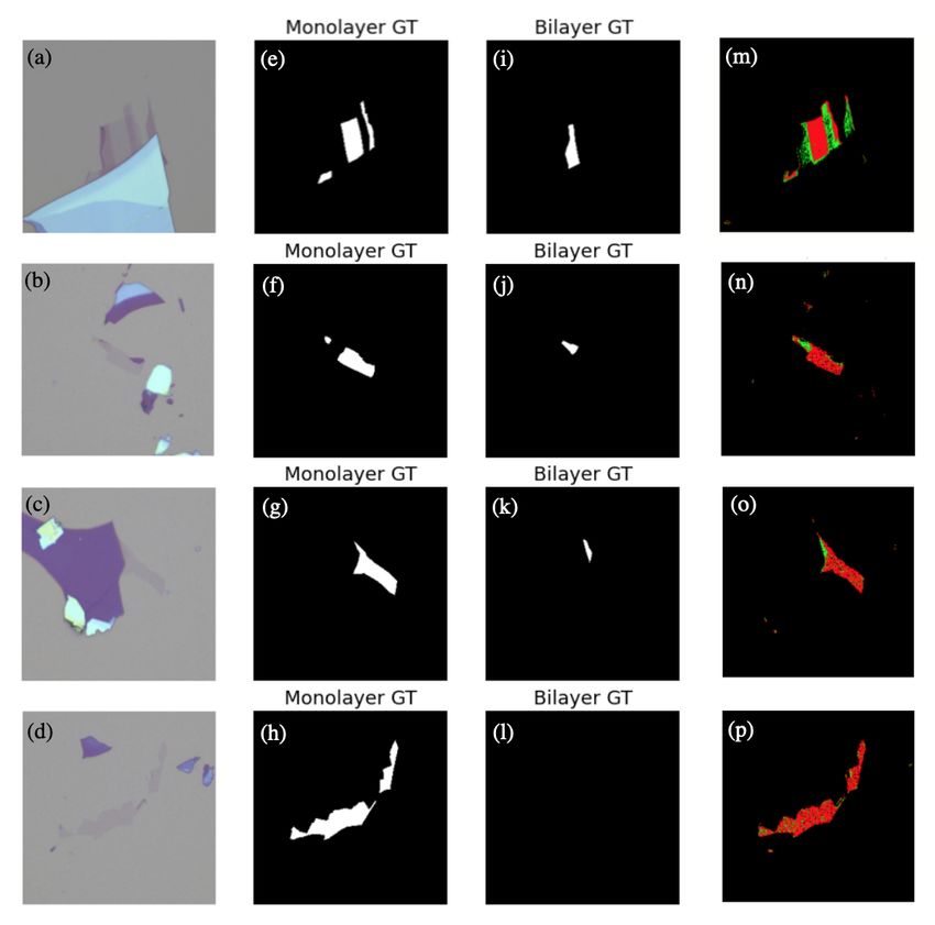
11]. In our work, the features on the dataset are limited. The shapes and the textures for graphene are not
      specific and thus we cannot include these two features in our training process. The only feature that we
      can apply to our training process is the color pixel values of graphene. In order to resolve this issue, we
      applied the SVM algorithm in MLA-GDCC as an image segmentation method to separate the monolayer
      and the bilayer graphene flakes from the regions of interest. Although the features in our dataset are very
      limited, the segmentation results for monolayer and bilayer graphene flakes show a high accuracy and a
      low FAR with the implementation of the SVM.

3     Machine Learning-based Automatic Graphene Detection Method with Color
      Correction (MLA-GDCC)
Fig. 1 shows the process of MLA-GDCC. First, we apply a WB method to the original images to correct
the color shifts caused by different cameras. Second, the modified U-Net architecture is used to segment the
regions of interest from the background in the white-balanced images. Third, a multiplier is implemented to
mask the background from the white-balanced images. Last but not least, a SVM is implemented to classify
the monolayer and bilayer graphene.

3.1   White Balance Method (WB)
Due to different types of the cameras used by different research groups to capture the graphene images, color
shifts can happen on the images. Therefore, we implement a WB correction in the MLA-GDCC method to
correct the color shifts. We implement a Gray world algorithm [4, 7, 17] as the WB method to make the
average of all channels a gray image. With the WB correction, models can accurately detect the graphene on
the color-shifted microscopic images captured by different cameras.

3.2   Modified U-Net architecture
In order to segment both the single layer and the bilayer graphene flakes from the background more accurately,
we modify the traditional U-Net architecture [29] by adding 5 convolutional layers in the decoder to generate
more training parameters from the images. The inputs of the modified U-Net are RGB microscopic images of
graphene on the SiO2 substrates, and all the input images are resized into 256 × 256 pixels. The outputs of the
modified U-Net are the detected masks containing both monolayer and bilayer graphene flakes, which provides
pixel-level probability maps for the graphene devices. The output of the modified U-Net is shown in Fig. 2. (b)
and (f) in Fig. 2 show the ground truths (GT) of the graphene flakes for both monolayer and bilayer graphene.
    We use the weighted binary cross-entropy defined below as the loss for the modified U-Net,
                                      1 1 X       (g)
                                 L=         (k · yi,j log(ȳi,j )+
                                      N h·w
                                                i,j                                                           (1)
                                                              (g)
                                                      (1 −   yi,j ) log(1   − ȳi,j )),

    where i,j are the pixel positions on each image, k represents the positive weight. Due to the data imbalance
of the number of pixels values between the background and the graphene flakes, positive weight is added here to
increase the weight of the positive samples, which are graphene pixel values. ȳi,j is the output of the modified
                                                                                            (g)
U-Net, N is the number of the images in the dataset, h is the height, w is the width and yi,j is the GT.

                                        ȳi,j = θ(wi,j,m,z · xz,m + bi,j ),                                   (2)
    In Eq. 2, θ stands for the activation function, here we implement a sigmoid function as the activation
function to confine the output values among [0,1]. wi,j,m,z is the weight, m and z are the input dimension
indexes, xz,m stands for the input of the neural network, bi,j is the bias.

                                                        3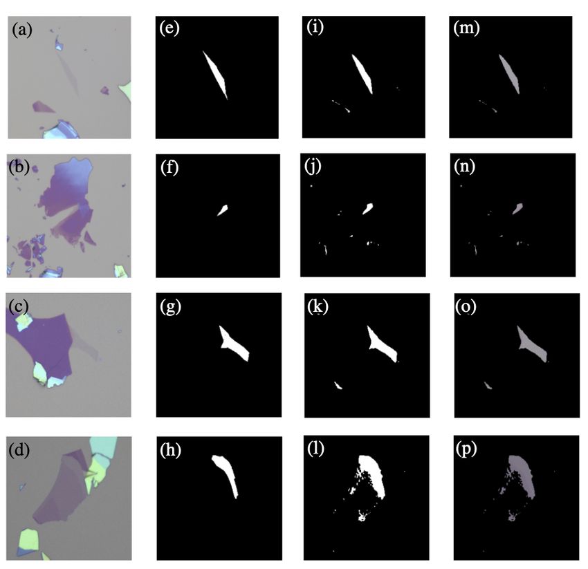
3.3     SVM: Color Pixels Classifier
A multiplier is implemented to mask the background in the white-balanced images as shown in Fig. 3. Only
the regions of interest on the white-balanced images are left at the output of the multiplier. The limited features
on the graphene dataset prevent the modified U-Net from classifying the monolayer and the bilayer graphene.
Therefore, we use a SVM to identify and classify the monolayer and bilayer graphene flakes more accurately.
SVM is a machine learning algorithm used to find the hyper-plane based on the dataset characteristics, this
algorithm aims to maximize the margin of the hyper-plane and the data points in a linear or a nonlinear case.
    A SVM has two criterias including the empirical error minimization and the control of model complexity.
With the two criteria, the cost function of the model can be minimized. The empirical error minimization
reduces the errors during the training to optimize the training result. The control of the model complexity can
prevent overfitting by controlling the flexibility of the function. The pixel intensity indicates the number of
layers of the graphene flakes.
    Here we extract the RGB pixel values separately and assign the pixel values to the corresponding label yi,j
indicating the layers of the graphene flakes. The features for the SVM algorithm include the mean values RGB
pixel values and the mean RGB pixel values of the mode background pixel values. By using the detection masks
from the U-Net, we use the histogram to select the peak value of the background for each R, G and B channel.
Next, we average the three background RGB pixel values to obtain the mean RGB pixel value as one of the two
features for the SVM algorithm. Since different images are composed of different mean pixel values, choosing
the background pixel value as one of the features is necessary to allow the SVM to identify the graphene flakes
more accurately. Given by the input dataset x, the discriminant function for a linear SVM can be defined by
                                                        N
                                                        X
                                            f (x) =           whx, xi i + b,                                   (3)
                                                        i=1

    where ω is a vector normal to the hyper-plane and b is a bias constant. However, the linear SVM cannot
find the optimized hyper-plane for the graphene flake classification. According to the Cover’s theorem [8], we
can adopt a nonlinear SVM to map x onto the higher dimensional space with the nonlinear mapping function,
φ(x). Therefore, the discriminant function for nonlinear SVM can be written as
                                                  N
                                                  X
                                        f (x) =         yi hφ(x), φ(xi )i + b,                                 (4)
                                                  i=1

where yi is the label of the training pattern xi , and N is the total number of training samples. The discriminate
function in Eq.4 is derived by minimizing the cost function defined as follows
                                                                        N
                                                    1            X
                                         C(ω, βi ) = ||w2 || + p   βi ,                                        (5)
                                                    2
                                                                        i=1

where βi denotes the distance to the correct margin βi ≥ 0. with the constraints are as follows:

                                   βi ≥ 1 − yi [ω · φ(xi ) + b], i = 1, 2, ..., N                              (6)

where

                                                βi ≥ 0 and C > 0                                               (7)

    where p is the regularization parameter, and βi are non-negative slack variables which are used to resolve
the noisy and nonlinearly separable data.
    And thus the decision function becomes

                                                g(x) = sgn[f (x)]                                              (8)

    According to the Mercer’s theorem [9, 15] the inner product in Eq. 3 can be replaced by a Kernel function
that is chosen for the dataset distribution.

                                         < φ(x), φ(xi ) > = K(xi , xj )                                        (9)

                                                              4
With the replacement of the Kernel function as shown in Eq. 9, we can rewrite the discriminate function as
the following equation:
                                                   N
                                                   X
                                         f (x) =         αi ωi K(x, xi ) + b,                                (10)
                                                   i=1

where K(x, xi ) represents the Kernel function. In our case, we select Gaussian Kernel to fit our dataset. The
Gaussian Kernel can be defined as follows:

                                     K(xi , xj ) = exp(−||xi − xj ||2 /2σ 2 )                                (11)

    With the implementation of the SVM algorithm, we can discriminate two classes in our dataset. The two
classes here are the monolayer and bilayer graphene mean RGB pixel values. The SVM algorithm does not
require a lot of training data. Although the training dataset is small, which in our case is 246 images, the model
achieves high detection rates of the monolayer and bilayer graphene flakes.

4     Experiments
4.1   Datasets and Implementation Environments
The dataset in this work is the graphene microscopic images obtained using mechanical exfoliation on top of
the SiO2 /Si wafers. The dataset includes 246 images for training and 57 images for testing. The height and
width of the images are both 256 pixels. The GTs are labeled manually by the authors using labelbox.com. The
GPU which is used to train the models in our work is a single 12GB NVIDIA Tesla K80 GPU.

4.2   Evaluation Metrics
We apply the evaluation metrics of Eqs. 12- 16 to evaluate the results from the SVM. In the equations, P stands
for graphene pixels and N stands for background pixels for the pixel-level evaluation metrics. For the flake-level
DR, TP stands for graphene flakes correctly detected, and FN stands for graphene flakes failed to be detected
by the model.

                                                                  TP
                                          Precision(%) =                .                                    (12)
                                                                TP + FP

                                                         2 · Precision · Recall
                                    F1 score(%) =                               .                            (13)
                                                          Precision + Recall

                                                                   TP
                                        Recall(DR)(%) =                  .                                   (14)
                                                                 TP + FN

                                                              TP + TN
                                   Accuracy(%) =                           .                                 (15)
                                                         TP + FN + TN + FP

                                                                     FP
                                      False alarm rate(%) =                .                                 (16)
                                                                   FP + TN

                                                           5
4.3   The Accuracy of MLA-GDCC
The training process of the modified U-Net is 450 epochs, with a learning rate of 0.001, and the positive weight
k of 200. We adopt the Adam optimizer [18] for training the modified U-Net. The modified U-Net is used to
separate the graphene flakes from the background. The pixel-level detection rate of the modified U-Net on the
test dataset is 97%, and the false alarm rate of the modified U-Net is 3%.
     We also compare the receiver operating characteristic (ROC) curves of the U-Net with and without the
additional 5 layers in Fig. 4. At the knee point of the curves we observe an improvement of the implementation
of the additional 5 convolutional layers added to the decoder. The detection rate at the knee point is increased
compared to the U-Net architecture. With a higher detection rate at the output using the modified U-Net, we
achieved an improvement of up to 0.7% in a detection rate of the modified U-Net compared to the original
U-Net.
     A multiplier is used to multiply the detected masks and the original images. Therefore, at the output of
the multiplier, the detected masks cover the background and only the graphene regions of interest are left.
The output from the multiplier are the input for the SVM. With the implementation of the SVM algorithm,
the monolayer and the bilayer graphene can be separated at the output of the SVM, as shown in Fig. 5. The
flake-level detection rates are 87.09% for monolayer and 90.41% for bilayer graphene.
     The pixel-level evaluation metrics for MLA-GDCC calculated using from Eq. 12 to Eq. 15 can be found in
Table 1. The precision is 51.01% for monolayer and 70.37% for bilayer graphene. The F1 score is 59.03% for
monolayer and 75.38% for bilayer graphene. The recall or detection rate is 70.05% for monolayer and 81.16%
for bilayer graphene. The accuracy is 99.27% for monolayer and 98.92% for bilayer graphene.

4.4   Ablation Study of White Balance Method
With the implementation of the Gray world algorithm, the results show that the SVM model can detect the
graphene flakes and identify the layers with high detection rates. The detection results of the color-shifted
images are shown in Fig.6 and Fig.7. In both Fig.6 and Fig.7, part (a) shows the images shifted with different
numbers of pixel values in the blue channel. Part (b) shows the application of the Gray world algorithm on the
images in part (a). Part (c) shows the output from the MLA-GDCC. The numerical results from the output of the
MLA-GDCC can be found in Table 2. We use the numerical results in Table 2 to plot Fig.8 and demonstrate the
detection rates with different shifted pixel values of the original images. With the WB correction applied to the
color-shifted images, the MLA-GDCC remains at high detection rates. The result shows how the robustness and
the reliability of the color correction method applied in the MLA-GDCC can deal with the potential color-shift
caused by different cameras.

5     Conclusions
In this paper, a MLA-GDCC method is introduced to automatically, precisely and rapidly classify monolayer
and bilayer graphene flakes. With the implementation of the Gray world algorithm, the color shifts on the
microscopic images caused by different cameras are resolved. We implement a modified U-Net architecture
and a SVM algorithm to achieve high detection rates of graphene flakes on the microscopic images. The MLA-
GDCC allows us to segment the graphene layers with high flake-level detection rates of 87.09% for monolayer
and 90.41% for bilayer graphene, and high pixel-level accuracy of 99.27% for monolayer and 98.92% for
bilayer graphene.

References
 [1] H. Alquran, I. A. Qasmieh, A. M. Alqudah, S. Alhammouri, E. Alawneh, A. Abughazaleh, and F. Hasayen. The
     melanoma skin cancer detection and classification using support vector machine. pages 1–5, 2017.
 [2] A. Balandin, S. Ghosh, W. Bao, I. Calizo, D. Teweldebrhan, F. Miao, and C. N. Lau. Superior thermal conductivity
     of single-layer graphene. Nano Letters, 8(3):902–907, 2008.
 [3] F. Bovolon, L. Bruzzone, and L. Carlin. A novel technique for subpixel image classification based on support vector
     machine. IEEE TRANSACTIONS ON IMAGE PROCESSING, 19:2983–2999, 2010.
 [4] G. Buchsbaum. A spatial processor model for object colour perception. 310:1–26, 1980.

                                                           6
[5] Y. Cao, V. Fatemi1, S. Fang, K. Watanabe, T. Taniguchi, E. Kaxiras, and P. Jarillo-Herrero1. Unconventional
superconductivity in magic-angle graphene superlattices. 556:43–50, 2018.
[6] O. Chapelle, P. Haffner, and V. N. Vapnik. Support vector machines for histogram-based image classification. IEEE
TRANSACTIONS ON NEURAL NETWORKS, 10:1055–1064, 1999.
[7] G. Chen and X. Zhang. A method to improve robustness of the gray world algorithm. pages 250–255, 2015.
[8] T. M. Cover. Geometrical and statistical properties of systems of linear inequalities with application in pattern
recognition. 14:326—-334, 1965.
[9] N. Cristianini and J. Shawe-Tayloi. An introduction to support vector machines. 2000.
[10] P. Gadosey, Y. Li, E. Agyekum, T. Zhang, Z. Liu, P. Yamak, and F. Essaf. Sd-unet: Stripping down u-net for
segmentation of biomedical images on platforms with low computational budgets. Diagnostics, 10(2), 2020.
[11] S. Hossain, R. Mou, M. Hasan, and and M. Razzak S. Chakraborty. Recognition and detection of tea leaf’s diseases
using support vector machine. 2018 IEEE 14th International Colloquium on Signal Processing and Its Applications
(CSPA), pages 150–154, 2018.
[12] J. Hu, D.Li, Q. Duan, Y. Han, G. Chen, and X. Si. Fish species classification by color, texture and multi-class support
vector machine using computer vision. Computers and Electronics in Agriculture, 88:133–140, 2012.
[13] Y. Huang, E. Sutter, N. N. Shi, J. Zheng T. Yang, D. Englund, H-J Gao, and P. Sutter. Reliable exfoliation of
large-area high-quality flakes of graphene and other two-dimensional materials. ACS Nano, 9(11):10612—-10620,
2015.
[14] M. Islam, Anh Dinh, K. Wahid, and P. Bhowmik. Detection of potato diseases using image segmentation and
multiclass support vector machine. pages 1–4, 2017.
[15] JMercer. Functions of positive and negative type and their connection with the theory of integral equations.
209:415—-446, 1909.
[16] V. Khryashchev, R. Larionov, A. Ostrovskaya, and A. Semenov. Modification of u-net neural network in the task
of multichannel satellite images segmentation. 2019 IEEE East-West Design Test Symposium (EWDTS), pages 1–4,
2019.
[17] Y. Kim, J-S Lee, A. Morales, and S-J Ko. A video camera system with enhanced zoom tracking and auto white
balance. IEEE Transactions on Consumer Electronics, 48:428–434, 2002.
[18] D. P. Kingma and J. Ba. Adam: A method for stochastic optimization. 2014.
[19] M. C. Lemme, T. J. Echtermeyer, M. Baus, and H. Kurz. A graphene field-effect device. IEEE Electron Device
Letters, 28:282–284, 2007.
[20] Y-M Lin and P. Avouris. Strong suppression of electrical noise in bilayer graphene nanodevices. Nano Letters,
8(8):2119–2125, 2008.
[21] A. Luican, G. Li, A. Reina, J. Kong andR. R. Nair, K. S. Novoselov, A. K. Geim, and E. Y. Andrei. Single-layer
behavior and its breakdown in twisted graphene layers. Phys. Rev. Lett., 106:126802, Mar 2011.
[22] L. Luo, D. Chen, and D. Xue. Retinal blood vessels semantic segmentation method based on modified u-net. pages
1892–1895, 2018.
[23] S. Masubuchi and T. Machida. Classifying optical microscope images of exfoliated graphene flakes by data-driven
machine learning. npj 2D Materials and Applications, 3(1):1–7, 2019.
[24] Edward McCann and Mikito Koshino. The electronic properties of bilayer graphene. Reports on Progress in Physics,
76(5):056503, 2013.
[25] K. S. Novoselov, A. K. Geim, S. V. Morozov, D. Jiang, Y. Zhang, S. V. Dubonos, I. V. Grigorieva, and A. A. Firsov.
Electric field effect in atomically thin carbon films. Science, 306(5696):666–669, 2004.
[26] K. S. Novoselov, A. Mishchenko, A. Carvalho, and A. H. Castro Neto. 2d materials and van der waals heterostruc-
tures. Science, 353(6298):aac9439, 2016.
[27] T. Ohta, A. Bostwick, T. Seyller, Karsten Horn, and Eli Rotenberg. Controlling the electronic structure of bilayer
graphene. Science, 313:951–954, 2006.
[28] J. G. G. S. Ramos, T. C. Vasconcelos, and A. L. R. Barbosa. Spin-to-charge conversion in 2d electron gas and
single-layer graphene devices. 123, 2018.
[29] O. Ronneberger, P.Fischer, and T. Brox. U-net: Convolutional networks for biomedical image segmentation.
9351:234–241, 2015.
[30] Eisuke S. Masubuchi, and Watanabe, Yuta Seo, Shota Okazaki, Takao Sasagawa, Kenji Watanabe, Takashi
Taniguchi, and Tomoki Machida. Deep-learning-based image segmentation integrated with optical microscopy
for automatically searching for two-dimensional materials. npj 2D Materials and Applications, 4(1):1–9, 2020.
[31] R. Saito, M. Hofmann, G. Dresselhaus, A. Jorio, and M. S. Dresselhaus. Raman spectroscopy of graphene and
carbon nanotubes. Advances in Physics, 60(3):413–550, 2011.
7[32] Y. Saito, K. Shin, K. Terayama, S. Desai, M. Onga, Y. Nakagawa, Y. Itahashi, Y. Iwasa, M. Yamada, and K. Tsuda.
Deep-learning-based quality filtering of mechanically exfoliated 2d crystals. npj Computational Materials, 5(1):1–6,
2019.
[33] K. Sakthivel, R. Nallusamy, and C. Kavitha. Color image segmentation using svm pixel classification image. IEEE
TRANSACTIONS ON IMAGE PROCESSING, 8:1924–1930, 2014.
[34] H. Seo, C. Huang, M. Bassenne, R. Xiao, and L. Xing. Modified u-net (mu-net) with incorporation of object-
dependent high level features for improved liver and liver-tumor segmentation in ct images. IEEE Transactions on
Medical Imaging, 39(5):1316–1325, 2020.
[35] A. Sevastopolsky. Optic disc and cup segmentation methods for glaucoma detection with modification of u-net
convolutional neural network. 27:618–624, 2017.
[36] C. Shearer, A. Slattery, A. Stapleton, J. Shapter, and C. Gibson. Accurate thickness measurement of graphene.
Nanotechnology, 27(12):125704, feb 2016.
[37] A. O. Vuola, S. U. Akram, and J. Kannala. Mask-rcnn and u-net ensembled for nuclei segmentation. pages 208–212,
2019.
[38] X-Y. Wang, T. Wang, and J. Bu. Color image segmentation using pixel wise support vector machine classification.
Pattern Recognition, 44:777–787, 2011.
[39] F. Xia, T. Mueller, Y-M Lin, A. Valdes-Garcia, and P. Avouris. Ultrafast graphene photodetector. Nature Nanotech-
nology, 4:839—-843, 2009.
[40] Y. Yang, C. Feng, and R. Wang. Automatic segmentation model combining u-net and level set method for medical
images. Expert Systems with Applications, 153:113419, 2020.
[41] Q. Yao, Z. Guan, Y. Zhou, J. Tang, Y. Hu, and B. Yang. Application of support vector machine for detecting rice
diseases using shape and color texture features. 2009 International Conference on Engineering Computation, pages
79–83, 2009.
[42] W. Yao, Z. Zeng, C.Lian, and H. Tang. Pixel-wise regression using u-net and its application on pansharpening.
312:364–371, 2018.
[43] Y. Zhang, and C. Girit T-T Tang, Z. Hao, M. Martin, A. Zettl, M. Crommie, Y. Shen, and F. Wang. Direct observation
of a widely tunable bandgap in bilayer graphene. Nature, 459:820–823, 2009.
Figure 1: Complete process of the MLA-GDCC.
8Figure 2: (a) and (e) are the original images. (b) and (f) are the GT masks. (c) and (g) are the outputs from the
modified U-Net architecture. (d) and (h) are the outputs from the modified U-Net architecture with a threshold.
Table 1: Pixel-level evaluation metrics
precision(%) F1 score(%) recall(DR)(%) accuracy(%)
Monolayer 51.01 59.03 70.05 99.27
Bilayer 70.37 75.38 81.16 98.92
Table 2: Flake-level detection rates changing with the shifted pixel values
Shifted pixel values -25 -20 -15 -10 -5 0 5 10 15 20 25
Monolayer DR(%) 82.25 82.25 85.48 87.09 87.09 87.09 87.09 87.09 87.09 87.09 82.25
Bilayer DR(%) 93.15 91.78 91.78 91.78 90.41 90.41 90.41 83.56 80.82 78.08 72.6
Table 3: Pixel-level detection rates and false alarm rates changing with the shifted pixel values
Shifted pixel values -25 -20 -15 -10 -5 0 5 10 15 20 25
Monolayer DR(%) 62.45 63.7 65.31 67.08 67.75 70.05 71.33 72.49 71.4 68.07 59.89
Bilayer DR(%) 81.63 81.11 80.92 81.4 80.81 81.16 80.15 74.32 74.54 68.55 66.46
Monolayer FAR(%) 0.41 0.45 0.47 0.48 0.51 0.51 0.56 0.68 0.7 0.77 0.8
Bilayer FAR(%) 0.75 0.73 0.66 0.72 0.71 0.71 0.69 0.68 0.74 0.76 0.76
9Figure 3: (a)-(d) are the original images. (e)-(h) are the GT masks. (i)-(l) are the outputs from the modified
U-Net. (m)-(p) are the outputs from the multiplier.
10Figure 4: ROC comparison between the U-Net and the modified U-Net architecture.
11Figure 5: (a)-(d) are the original images. (e)-(h) are the ground truth images of the monolayer graphene. (i)-
(l) are the ground truth images of the bilayer graphene. (m)-(p) are the detected monolayer(green area) and
bilayer(red area) graphene.
12Figure 6: (a) shows the original images with the pixel values in the blue channel subtracted with the correspond-
ing values on the images. (b) shows the images after applying white balance on (a). (c) shows the detection
results from the SVM.
Figure 7: (a) shows the original images with pixel values in the blue channel added with the corresponding
values on the images. (b) shows the images after applying white balance on (a). (c) shows the detection results
from the SVM.
13Figure 8: Detection rates of the input images shifted with different pixel values.
14You can also read