Designing real-time traffic management for an urban rail transit system - London's new Elizabeth line, UK

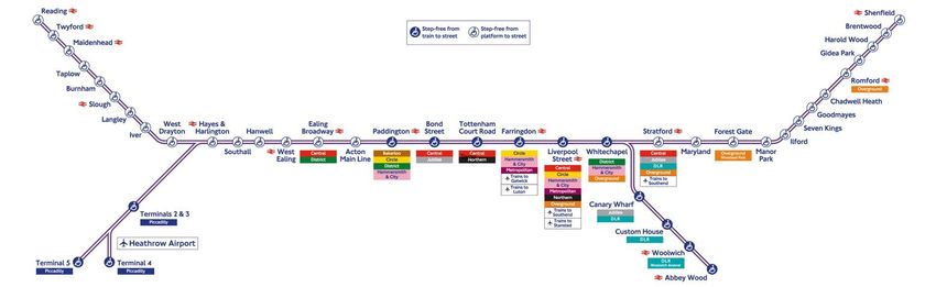
INFORMS Railway Applications Section
2022 Problem Solving Competition
Problem description
Version 2.3

Designing real-time traffic management for
an urban rail transit system – London’s new
Elizabeth line, UK
1 Problem description
As a global rail operator, MTR is working with TrenoLab in the development of a state of the art
Decision Support Tool, which will be used in helping build resilience into London’s new railway –
the Elizabeth line.

The Elizabeth line (formally known as Crossrail) will stretch more than 60 miles from Reading and
Heathrow in the west through central tunnels across to Shenfield and Abbey Wood in the east. It
will ultimately provide a seamless transit service between the East and West parts of the British
capital city, with several connections to the railway and underground networks, as well as with the
Heathrow international airport.

The rail network features the shape of an “horizontal X”, with four extremity terminals: Reading
and Heathrow airport on the West side, and Abbey Wood and Shenfield on the East one. Planned
services will originate/terminate from/at these terminals as well as from intermediate stations. An
illustration of the network is provided by Figure 1.

At the full planned regime, more than 1000 daily trains will be operated by the Train Operating
Company (TOC) MTR Elizabeth line on behalf of Transport for London (TfL), resulting in a
minimum service headway (time between consecutive trains in the same direction) of 150 s in the
central section of the network, where all services between different origins/destinations share the
same tracks. In this part of the network a Communication Based Train Control system will allow for
a nominal minimum technical headway of about 90 s, while in the peripheric branch a conventional
signaling system will allow for an approximate minimum technical headway of 240 s.

Figure 1. The Elizabet line.

On a such densely used system, even minor disturbances, especially during peak hours, could result
in major implications on the planned timetable and rapid delay spread and potential service
cancellations because of two main factors:
 • Congestion in the central section;
 • Strong interweaving of courses at terminal stations due to rolling stock circulation.

Timetable disruptions ultimately result in a loss of service quality for passengers, for which the
TOC will have to pay an economic fee. A set of penalty KPIs is defined to this purpose, in general
depending on time and space (e.g., scarcely frequented stations during off-peak hours accounts less
than heavily used ones in peak hours).

To maintain a given level of service, and thus, to minimize the economic penalty to be paid, the
TOC can perform an active dispatching of the traffic, resulting in a set of timetable amendments.
Timetable amendments are actions which modify the planned timetable in real-time during
operations. Therefore, from that time on, trains will have to run following the amended timetable
instead of the originally planned one. In general, amendments do not come free, meaning that they
do involve a certain amount of penalty. Possible amendments could be train retiming, choosing a
different platform, skipping a stop, cancelling a service. An effective amendment set is that which
involves a total penalty (computed on the amended timetable) minor than the penalty to be paid in
case of no amendments are applied.

Finally, amendments must be designed in such a way that they ensure a feasible rolling stock
circulation, possibly resorting to calls for available reserve units in depots.

The aim of the competition is to develop a method to compute the optimal sets of amendments for a
given set of timetable disruption scenarios using a Decision Support Tool. A disruption can be
caused by disturbances of traffic as well as speed reductions on railway track.

Section 2 introduces the input data, which are then discussed in detail in subsequent sections.
Section 3 describes the model for infrastructure and timetable. Section 4 explains how the
disruptions are structured and described. Section 5 illustrates possible amendment types while
Section 6 deals with the computation of the economic penalties. Finally, Section 7 describes the
objective of the competition including the expected deliverables.

2 Input data
The input dataset provided to participants is composed by:
 · A planned daily timetable;
 · The planned rolling stock duties;
 · Infrastructure data, i.e., minimum run times and headways (minimum time separation
 between two trains) for the concerned rolling stock type on the considered network;
 · A set of problem instances. Each instance is a disrupted timetable, which is qualified by the
 realized timetable until a certain time and by a set of conditions such as slowdowns which
 are expected to occur after that time. These conditions are potential causes of additional
 delays which must be properly handled.
 · A set of KPIs for computing the economical penalty due to actual traffic diverging from the
 planned timetable. These KPIs consider:
 o Skipped stops;
 o Destination delays;
 o Headways in the central section of the network, between Whitechapel and
 Paddington.

The data is in two equivalent formats, an Excel spreadsheet and a Microsoft Access database. Both
formats were provided to make it easier to use, and both formats can be read in from various
languages (e.g., Python, R, C#) and environments (Windows and Linux). A formal data dictionary
is in the Excel spreadsheet.

3 Infrastructure/timetable model
3.1 General assumptions
Due to the nature of the considered case study, we can adopt the following simplifications:
 • One type of rolling stock only (345 class EMUs) is used for the all considered services and
 for the empty moves to/from depots. Split-and-join operations (more than one EMUs
 operating the same train) are not considered.
 • The whole considered network is double-track. Certain stations may have more than two
 tracks. Part of the problem should consider maintenance-of-way considerations when a
 section of double track is reduced to a single track for a limited time.
3.2 Infrastructure model
We adopt a macroscopic model for infrastructure and operations, based on a graph = ( , ).

Nodes are the macroscopic timing locations (stations, junctions, halts and control points) in the rail
network.

The nodes are found in the NODE table. Table 1 is a relevant small example.
Table 1. Example of the NODE table.
 NODE
 NAME CODE CATEGORY EB_TRACKS WB_TRACKS LATITUDE LONGITUDE
 BOND STREET BONDST STATION 2 1 51.514299 -0.149002
 FISHER ST EAST FRNDFST STATION 2 1 51.520161 -0.104616
 FARRINGDON CROSSRAIL FRNDXR STATION 2 1 51.520280 -0.098256
 LONDON LIVERPOOL STREET LIVST STATION 17 17 51.518166 -0.081768
 LIVERPOOL ST CROSSRAIL LIVSTLL STATION 1 2 51.517409 -0.082537
 PADDINGTON CROSSRAIL PADTLL STATION 1 2 51.519868 -0.177073
 LONDON PADDINGTON PADTON STATION 11,12 11,12 51.517702 -0.178155
 FISHER ST WEST TOTCFST STATION 2 1 51.520780 -0.107688
 TOTTENHAM COURT ROAD TOTCTRD STATION 2 1 51.516269 -0.130838
 WHITECHAPEL CROSSRAIL WCHAPXR STATION 2 1 51.519470 -0.057691
 VALENCE ROAD WCHAVRD STATION 2 1 51.518384 -0.062900

The CODE field will be used throughout the remainder of the data and will be called NODE in
other tables. As a side note, this field is internally called TIPLOC.

The node category field was supplied as information. A STATION is node where a train can
pickup/drop off passengers. One use of this field is to help the user creates network graphs that
display nodes with different formats depending on the node category.

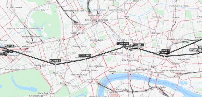
Figure 2. Georeferenced example of the Elizabeth line network in central London.

The name, latitude and longitude are useful for locating the nodes on a map. Figure 2 provides a
relevant example located in central London.
For each node we define:
 • A set of tracks for each direction. Each track is identified by a comma separated
 alphanumeric string, unique within each station;
 • A minimum separation time between the end of the occupation of a track by a train and the
 beginning of the occupation of the same track by the following one ℓ , providing that each
 track can be used by at most one train at a time.

Edges connect adjacent nodes and are in the LINK table. A relevant example is provided by Table
2.
Table 2. LINK table example.
 START_NODE END_NODE DIRECTION DISTANCE_METERS
 BONDST PADTLL WB 250
 BONDST TOTCTRD EB 1034
 FRNDFST FRNDXR EB 1064
 FRNDFST TOTCFST WB 81
 FRNDXR FRNDFST WB 1064
 FRNDXR LIVSTLL EB 1166
 LIVST WHELSTJ EB 250
 LIVSTLL FRNDXR WB 1166
 LIVSTLL WCHAVRD EB 1675
 PADTLL BONDST EB 250
 PADTLL ROJAOJN WB 250
 PADTON ROYAOJN WB 250
 TOTCFST FRNDFST EB 81
 TOTCFST TOTCTRD WB 1112
 TOTCTRD BONDST WB 1034

TOTCTRD TOTCFST EB 1112
 WCHAPXR WCHAVRD WB 341
 WCHAVRD LIVSTLL WB 1675
 WCHAVRD WCHAPXR EB 341

Notice that for every adjacent pair of nodes, there are two edges. For example, BONDST and
PADTLL are adjacent. There is a BONDST to BONDST link in the westbound direction and a
BONDST to BONDST link in the eastbound direction. In both directions, the distance (in meters)
is the same.

A few edges are denoted as having direction BOTH. These are for edges that have a degree-1 end
and that trains could leave from that end to other parts of the network in either direction.
A train can cross each extremity node with two different activities, i.e. passing or stopping. The
running time on an edge depends on the activities at the corresponding nodes, i.e. pass/pass,
pass/stop, stop/pass, stop/stop. It is assumed that a train can stop only on nodes, i.e. stops within
edges are neglected.

On an edge we have a technical minimum run time depending on the direction it is travelling
(which is implicit in the LINK_START_NODE/LINK_END_NODE and on the pair of activities in
the extremity nodes. Table 3 provides an example from the MINIMUM_RUN_TIME table. In this
example, it appears that each stop increases the run time by 15 seconds, although that is not a firm
rule everywhere in the network so this table must be used.

Table 3. MINIMUM_RUN_TIME table example.
 MINIMUM RUN
 LINK_START_NODE LINK_END_NODE START_ACTIVITY END_ACTIVITY TIME SECONDS
 TOTCFST FRNDFST PASS PASS 4
 TOTCFST FRNDFST PASS STOP 19
 TOTCFST FRNDFST STOP STOP 34
 TOTCFST FRNDFST STOP PASS 19
 FRNDFST TOTCFST PASS PASS 6
 FRNDFST TOTCFST PASS STOP 21
 FRNDFST TOTCFST STOP STOP 36
 FRNDFST TOTCFST STOP PASS 21
 PADTLL BONDST PASS PASS 150
 PADTLL BONDST PASS STOP 165
 PADTLL BONDST STOP STOP 180
 PADTLL BONDST STOP PASS 165
 BONDST PADTLL PASS PASS 150
 BONDST PADTLL PASS STOP 165
 BONDST PADTLL STOP STOP 180
 BONDST PADTLL STOP PASS 165

There is also a minimum head-to-head headway between the entrance time of a pair of consecutive
trains running in the same direction. It depends on the activities pair of each train in the end nodes
of the edge. Table 4 provides a relevant example. Examining the eighth line below, if a train goes
through PADTLL but does not stop, and then stops at ROJAOJN, then moves on, and the train
behind it going also in the same direction stops at PADTLL and then stops at ROJAOJN, then there

has to be at least 90 seconds between when the first train leaves PADTLL and the train behind it
enters PADTLL.
Table 4: Example of MINIMUM_HEADWAY table.
 START END START END
 ACTIVITY ACTIVITY ACTIVITY ACTIVITY MINIMUM
 TRAIN TRAIN TRAIN TRAIN HEADWAY
 LINK_START_NODE LINK_END_NODE FRONT FRONT BEHIND BEHIND SECONDS
 PADTLL ROJAOJN PASS PASS PASS PASS 90
 PADTLL ROJAOJN PASS PASS PASS STOP 90
 PADTLL ROJAOJN PASS PASS STOP PASS 90
 PADTLL ROJAOJN PASS PASS STOP STOP 90
 PADTLL ROJAOJN PASS STOP PASS PASS 90
 PADTLL ROJAOJN PASS STOP PASS STOP 90
 PADTLL ROJAOJN PASS STOP STOP PASS 90
 PADTLL ROJAOJN PASS STOP STOP STOP 105
 PADTLL ROJAOJN STOP PASS PASS PASS 90
 PADTLL ROJAOJN STOP PASS PASS STOP 90
 PADTLL ROJAOJN STOP PASS STOP PASS 90
 PADTLL ROJAOJN STOP PASS STOP STOP 90
 PADTLL ROJAOJN STOP STOP PASS PASS 105
 PADTLL ROJAOJN STOP STOP PASS STOP 105
 PADTLL ROJAOJN STOP STOP STOP PASS 105
 PADTLL ROJAOJN STOP STOP STOP STOP 105

3.3 Timetable and Rolling Stock Duties
Each course (i.e. a train scheduled in the planned timetable) is characterized by:
 • A unique COURSE_ID;
 • A nominal direction within the network, being it “Eastbound” (EB) or “Westbound” (WB);
 • A category, either “OO” (passenger service) or “EE” (empty/non-revenue ride).
Table 5 provides an example from the TRAIN_HEADER table. Note that the start/end of the
seconds/nodes are derived from the timetable described below.
Table 5. Example of the TRAIN_HEADER table.
 TRAIN START END START END
 COURSE_ID DIRECTION CATEGORY SECONDS SECONDS NODE NODE
 2C15RT#1 WB OO 21120 22980 GIDEAPK LIVST
 2N02RW#1 WB OO 83580 86100 PADTON MDNHEAD
 2R01RT#1 WB OO 25200 28440 PADTON RDNGSTN
 2T01RT#1 WB OO 18720 20400 PADTON HTRWTM5
 2W01RW#1 WB OO 84360 86880 SHENFLD LIVST
 2W02RW#1 EB OO 87540 90000 LIVST SHENFLD
 9U79RX#1 EB OO 73440 74220 PADTLL WCHAPXR

The actual train schedule – also called a ‘course’ – shows the nodes the train passes through and the
arrival and departure times. This is found in the table SCHEDULE. Table 6 reports an example for
one train that starts in PADTLL and ends at SHENFLD, travelling along some of the nodes
displayed in Figure 2 (not all the nodes are displayed in the example table).

Table 6. Example of the SCHEDULE table.
 TRAIN ARRIVAL ARRIVAL DEPARTURE DEPARTURE
 COURSE ID SEQ NODE SECONDS HHMMSS SECONDS HHMMSS TRACK ACTIVITY
 9W54RN#1 1 PADTLL 60780 16:53:00 1 STOP
 9W54RN#1 2 BONDST 60930 16:55:30 60960 16:56:00 2 STOP
 9W54RN#1 3 TOTCTRD 61020 16:57:00 61080 16:58:00 2 STOP
 9W54RN#1 4 TOTCFST 61153 16:59:13 61153 16:59:13 2 PASS
 9W54RN#1 5 FRNDFST 61159 16:59:19 61159 16:59:19 2 PASS
 9W54RN#1 6 FRNDXR 61230 17:00:30 61290 17:01:30 2 STOP
 9W54RN#1 7 LIVSTLL 61380 17:03:00 61440 17:04:00 1 STOP
 9W54RN#1 8 WCHAVRD 61539 17:05:39 61539 17:05:39 2 PASS
 9W54RN#1 9 WCHAPXR 61560 17:06:00 61590 17:06:30 2 STOP
 …
 9W54RN#1 29 SHENLEJ 63977 17:46:17 63977 17:46:17 1 PASS
 9W54RN#1 30 SHENFLD 64020 17:47:00 5 STOP

Note this is an ordered table that shows the route of the train and gives the arrival time and
departure time for each node within the route. The first node has an empty arrival time and the last
node has an empty departure time.

The locations that are passed through would have arrival time = departure time. The stations that
the train stops at will have a positive dwell time.

The track refers to the track at the node that the normal schedule will use. Given the direction of
the train, this almost always one of the tracks listed in the NODE table. Occasionally, this track is
not listed in the column of the NODE table for the train direction. Typically, this is for short empty
trains that use the tracks in the opposite direction.

Note times are given two ways. One is the number of seconds from midnight. There are 86400
seconds in a day, and occasionally the train activity is early in the next day and the time will be
greater than 86400. There is also a string format of the time. For those times when it goes to the
next day, there is a prefix of “1d” added to the time.

The last table shows the intended set of duties for a single train set (also called rolling stock) and is
called ROLLING_STOCK_DUTY.

This table shows how the train set is cycled through the network, from the first use of the train set
that day to the last use. Note that every moment between the first use and last use is accounted for.
Each row of the table is some type of event. There are 4 types of events:
▪ TRAIN: the rolling stock is operating a course (either a OO/passenger train schedule or an
 EE/empty train schedule),
▪ CHANGE_END: minimum technical time required by terminal operations. It can typically span
 between 60 s (without cabin turn-over) and 420 s (with cabin turn-over),
▪ SPARE: “free” time (can be reduced down to 0 if needed).
▪ RESERVE, which indicates the rolling stock is sitting idle and can be placed into use to support
 a timetable amendment.
 ▪ This ‘hot-reserve’ duties can be used to manage duties disruptions. The START_NODE
 indicates the depot at which the reserve is homed.

Note that the TRAIN events feature a START_NODE different from the END_NODE, since they
represent a movement of the rolling stock. The other events will always have START_NODE and
END_NODE being the same. However, in every case END_TIME_SECONDS >
START_TIME_SECONDS.

Table 7 reports an example of a complete duty.
Table 7. Example from the ROLLING_STOCK_DUTY table.
 START START END END
 TIME TIME TIME TIME START END EVENT TRAIN
 DUTY_ID SEQ SECONDS HHMMSS SECONDS HHMMSS NODE NODE TYPE COURSE_ID
 RSDuty_29 1 70920 19:42:00 71580 19:53:00 OLDOXRS PADTLL TRAIN 5U75RX#1.A1
 RSDuty_29 2 71580 19:53:00 71640 19:54:00 PADTLL PADTLL CHANGE_END
 RSDuty_29 3 71640 19:54:00 73380 20:23:00 PADTLL ABWDXR TRAIN 9U75RX#1.A1
 RSDuty_29 4 73380 20:23:00 73800 20:30:00 ABWDXR ABWDXR CHANGE_END
 RSDuty_29 5 73800 20:30:00 77760 21:36:00 ABWDXR HTRWTM5 TRAIN 9T54RV#1.A1
 RSDuty_29 6 77760 21:36:00 78180 21:43:00 HTRWTM5 HTRWTM5 CHANGE_END
 RSDuty_29 7 78180 21:43:00 78720 21:52:00 HTRWTM5 HTRWTM5 SPARE
 RSDuty_29 8 78720 21:52:00 82680 22:58:00 HTRWTM5 ABWDXR TRAIN 9U79RV#1.A1
 RSDuty_29 9 82680 22:58:00 83100 23:05:00 ABWDXR ABWDXR CHANGE_END
 RSDuty_29 10 83100 23:05:00 83580 23:13:00 ABWDXR ABWDXR SPARE
 RSDuty_29 11 83580 23:13:00 87720 1d 00:22:00 ABWDXR MDNHEAD TRAIN 9N92RV#1.A1
 RSDuty_29 12 87720 1d 00:22:00 87840 1d 00:24:00 MDNHEAD MDNHEAD CHANGE_END
 RSDuty_29 13 87840 1d 00:24:00 87960 1d 00:26:00 MDNHEAD MDNHDCS TRAIN 5N92RV#1.A1

For your convenience, we added a computed table ALL_DUTY_START_END. This table
summarizes the ROLLING_STOCK_DUTY to have one line by DUTY_ID to show the starting
node, ending node of the set of duties corresponding to a single DUTY_ID. It also shows when the
starting and ending time in seconds from midnight.

When you study this table, it is apparent that node-balance is not met. For example, there are four
more DUTY_IDs that end in MDNHEAD by the end of the day than start there in the morning.
Likewise, there are five more DUTY_ID’s that start at RDNGSTN than end them. Sometime
between 0100 and 0400, crews will ‘ferry’ these train sets to locations that need them. Most likely,
the 4 extra train sets that end up at MDNHEAD will be ferried to RDNGSTN.
In the below sample of ALL_DUTY_START_END, we have proposed ferry’s to bring all the train
sets into balance.

Note: you should not worry about imbalances at the end of the night – it is always possible to ferry
the train sets to be in the proper position the next day.

Table 8. Example from the ALL_DUTY_START_END table.
 DUTY_ID START_TIME_SECONDS START_NODE END_TIME_SECONDS END_NODE
 FERRY_1 7200 MDNHDCS 7245 MDNHDRS
 FERRY_2 7620 MDNHEAD 7838 RDNGSTN
 FERRY_3 8040 MDNHEAD 8258 RDNGSTN
 FERRY_4 8460 MDNHEAD 8678 RDNGSTN
 FERRY_5 8880 MDNHEAD 9098 RDNGSTN
 FERRY_6 9300 HTRWTM4 11009 OLDOXRS
 FERRY_7 9720 HTRWTM4 12014 RDNGSTN

FERRY_8 10140 SHENFLD 10163 SHENFMS
 FERRY_9 10560 PLMSXCR 12331 WBRNPKS
 RSDuty_1 26700 GIDEPKS 33060 GIDEPKS
 RSDuty_10 46620 OLDOXRS 87900 SHENFLD
 RSDuty_11 21000 ILFEMUD 80340 OLDOXRS
 RSDuty_12 58200 RDNGSTN 82260 MDNHDCS
 RSDuty_13 19320 MDNHDCS 81240 OLDOXRS
 RSDuty_14 15660 OLDOXRS 72660 MDNHEAD

3.3.1 Rolling Stock Connections
Throughout the day at several nodes the rolling stock terminates its set of duties, and is stored
within that node.
Below is a graph showing how many train sets are being stored at Gidea Park (GIDEPKS). We see
from around 0200 to 0445 there are 9 train sets. At about 0615, there are 3 train sets. One of them
pulls out to go onto a duty. We are not worried about which one of the three train sets is used. We
will impose a 7 minute (420 second) minimum connection time between these train sets. As soon
as one completes its set of duties at a node, it must wait at least 7 minutes before being used for
another DUTY_ID.

3.3.2 Rolling Stock Duty Feasibility Requirements
When constructing timetable amendments, sometimes it would cause disruptions in the planned
duties, which must be properly managed. Possible changes to the duties include:
 1. Swap some components of two duties, to draw a reserve unit from a depot (if any reserve is
 available) or to send a unit to a depot. In any case, each time a new CHANGE_END
 component has to be scheduled in an amended duty, a default time of 420 s must be used.
 2. In case of drawing/sending a unit from/to a depot, a new empty ride will be scheduled. The
 set of available depots is composed by all the locations in which planned duties originate or
 end. Capacity of depots is neglected, i.e. there is no limit to the number of units that can
 reside in same depot at the same time.

4 Problem instances
A problem instance is characterized by:
 • The realized schedule until time t, possibly with some trains running late with regard to the
 planned schedule;
 • A set of “known future incidents” occurring after time t. These incidents are causes of
 potentially serious delays which are already expected to occur at the time at which
 amendments are planned.
Problem instances are provided by means of Excel files. Different worksheets provide information
about the realized timetable and the future incidents.

The worksheet REALIZED_SCHEDULE describes all the timetable events occurred before time t,
in terms of actual arrival/departure times up to the last crossed node. Its structure is similar to that
of table SCHEDULE in the input dataset, with the difference that only trains departing before or at
time t will appear. Fields referring to events still not realized are left blank.

Table 9 provides an example for train 9W54RN#1, taken at time 17:05:00. At this time the train is
still running between LIVSTLL and WCHAVRD, so the last recorded event is the departure from
LIVSTLL at 17:04:00. In the example, train 9W54RN#1 is basically running on time, yet some
minor deviations from the planned timetable are present.

The actual track column is not always populated if there is only one real choice for the track. For
example, the last known position of the train is at LIVSTLL. This is an eastbound train, and there is
only one choice of track (track 1) at LIVSTLL going eastbound, and in that case it is left blank.

Knowledge of the track maybe helpful for those trains that have not yet left the station.

Table 9. Example of the REALIZED_SCHEDULE table.
 REAL. REAL. REAL. REAL. ACTUAL
 TRAIN ARRIVAL ARRIVAL DEPARTURE DEPARTURE TRACK
 COURSE_ID SEQ NODE SECONDS HHMMSS SECONDS HHMMSS
 9W54RN#1 1 PADTLL 60781 16:53:01 1
 9W54RN#1 2 BONDST 60918 16:55:18 60968 16:56:08
 9W54RN#1 3 TOTCTRD 61056 16:57:36 61106 16:58:26
 9W54RN#1 4 TOTCFST 61158 16:59:18 61158 16:59:18
 9W54RN#1 5 FRNDFST 61161 16:59:21 61161 16:59:21
 9W54RN#1 6 FRNDXR 61236 17:00:36 61290 17:01:30
 9W54RN#1 7 LIVSTLL 61382 17:03:02 61440 17:04:00
 9W54RN#1 8 WCHAVRD
 9W54RN#1 9 WCHAPXR
 …
 9W54RN#1.A1 30 SHENFLD

Four types of incidents are considered. In the following, they are further described, also with the
aid of examples consistent with an “amendment time” set at 17:05:00.

NOTE: In the actual database times will be given both as a number of seconds from midnight, as
well as a string in the format HH:MM:SS or possibly 1d HH:MM:SS for those times past midnight.

4.1 Extended run times on an edge
This incident imposes that on edge (direction given by the start/end node) within a given time band,
all trains (independently from their rolling stock) must travel with an extended running time
significantly greater than the planned one.
Example: Because of planned works alongside the tracks between 17:10:00 and 18:10:00, trains
will take 4 minutes to travel from TOTCTRD to BONDST, instead of the planned 1.5 minutes.
Relevant data:
 • Start/end nodes;
 • Start and end times;
 • Extended run time

Sample table (EXTENDED_RUN_TIMES worksheet):
 START START EXTENDED
 START TIME TIME END TIME END TIME RUN TIME
 NODE END NODE SECONDS HHMMSS SECONDS HHMMSS (s)
 TOTCTRD BONDST 61800 17:10:00 65400 18:10:00 240

4.2 Late departure from depot
This incident imposes that a course planned to leave from its initial node actually departs with a
delay.

NOTE: the time when the course departs from its first node should be after the amendment time.

Example: Course 5U67RN#1 is planned to depart from OLDOXRS (Old Oak Depot) at 17:14:00.
At the amendment time 17:05:00 the driver assigned to this course communicates to the dispatching
center that he is late and will arrive at the depot not before 17:10:00. Then the dispatcher forecasts
that course 5U67RN#1 will depart at 17:25:00, with a delay of 11 minutes.
Relevant data:
 • Course id;
 • Departure delay in seconds

Sample table (LATE_DEPARTURES worksheet):
 DEPARTURE
 COURSE_ID DELAY (s)
 5U67RN#1 660

4.3 Extended dwell time for all trains stopping at a station
This incident imposes that all courses stopping at station within a time band will be subject to a
dwell time significantly greater than the planned one.
Example: Due to a sport event, it is expected that all trains calling at BONDST between 18:00:00
and 18:20:00 will stop 2 minutes instead of the planned stop time.
Relevant data:
 • Node;
 • Start and end times;
 • Extended dwell time;

Sample table (STATION_EXT_DWELL worksheet):
 START START
 TIME TIME END TIME END TIME EXT DWELL
 NODE SECONDS HHMMSS SECONDS HHMMSS TIME (s)
 BONDST 64800 18:00:00 66000 18:20:00 120

4.4 Extended dwell time for a train at a station
This incident imposes that a course at a node will be subject to a dwell time significantly greater
than the planned one.
Example: Course 9T58RN#1 is running on time, and is planned to arrive at LIVSTLL at 17:05:30
and stop there 1 minute. At 17:05:00, while approaching the stop, the driver communicates to the

dispatching center that an ill passenger is onboard. It is then forecasted that the course will stop at
the next station LIVSTLL for 6 minutes to assist the ill passenger.
Relevant data:
 • Course id;
 • Node;
 • Extended dwell time in seconds

Sample table (TRAIN_EXT_DWELL worksheet):
 EXT DWELL
 COURSE ID NODE TIME (s)
 9T58RN#1 LIVSTLL 360

5 Timetable amendments
A timetable amendment is an active modification of the planned timetable. We consider the
following types of basic amendments:
 · Re-timing of courses in station st: planned arrival/departure (stop) times are modified
 within given ranges;
 · Re-platforming of courses in station st: planned station track is modified, considering the
 set of available tracks for that course in that station specified in input data;
 · Skipped stop in station st: a train passes through st instead of stopping as in the planned
 timetable;
 · Partial cancellations in station st: a course is “cut” at an intermediate location.
 · Total cancellations: a course is not operated at all.

Some timetable amendments imply the disruption of one or more rolling stock duties, which must
be amended too. For instance, a train running late may miss a connection with the following course
in the relevant rolling stock duties. Normally, it is desired that the following course departs on time,
in order to avoid propagation of delay. Cancellations (partial or total) would in most cases produce
a rolling stock duty disruption as well, which can be managed, for instance, by calling a reserve unit
from a depot. In general, the following actions can be performed to amend disrupted rolling stock
duties:
 · Send a unit to a depot;
 · Draw a unit from a depot;
 · Schedule empty rides between different stations;
 · In case of partial cancellation, short-turning a pair of courses: the unit of the “cut” course
 waits on a station tracks and “catch” the path of the following connected course in the duty.
 This implies a partial cancellation of the connected course as well (see Figure 3);

Figure 3. Short-turning at station st, resulting in partial cancellations of courses A1 and B1.

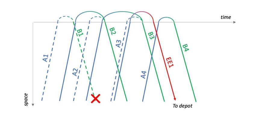
· Adjust rolling stock circulation at station st: some rolling stock duties are modified in
 order to avoid propagation of delays, at the price of cancelling a course. Figure 4 provides a
 graphical example, where planned paths are depicted by a dashed line while actual ones by a
 solid line. Courses A1, A2 and A3 arrive at a terminal station with certain amount of delay.
 In order to prevent delay propagation from the perturbed course A1 to the connected courses
 B1, B1 is cancelled and the rolling stock of A1 will operate course B2, which will depart
 on-time. Subsequently, material of course A2 will operate course B3, and finally the rolling
 stock of course A3 is sent to depot as a newly-created empty ride EE1 since course A4 is
 running on-time and there is no longer need to shift the duties. The figure also highlights the
 need for more than one available station track to operate this amendment. Courses can use
 the station tracks provided as input data.

Figure 4. Graphical example of a rolling stock re-circulation at terminal.

6 Penalty computation
6.1 Skipped stops
For each course of category OO, each planned stop which is skipped in the amended timetable will
involve an economic penalty, depending on the station and on the time.
Total and partial cancellations are evaluated considering the resulting set of skipped planned stops.
For instance, the total cancellation of a course result in a set of skipped stops equal to the set of the
planned stops for that course.
In general, let be the set of skipped stops for course . The resulting penalty for course called
 , is calculated as

 , = ∑ ( ) ∙ ( )
 ∈ 

 ( ) is the Base Station Value in £ and depends on:
 • The nominal direction of the course ;
 • The station at which the skipped stop takes place;
 • The planned arrival time for course and the concerned station.

Base Station Values are defined by two tables (one for each nominal direction, provided in the
Attachments), of which Table 10 provides a relevant example.

Table 10. Example of a Base Station Values table.
Westbound (WB) Timebands
 Start
 06.06- 07.00- 07.45- 09.15- 10.00- 16.00- 16.45- 18.15- 19.00- 21.00- 24.00-
Station to
 06.59 07.44 09.14 09.59 15.59 16.44 18.14 18.59 20.59 23.59 End
 06.05
SHENFLD 96 72 120 144 120 72 90 108 90 72 72 96
BRTWOOD 128 96 160 192 160 96 120 144 120 96 96 128
HRLDWOD 96 72 120 144 120 72 90 108 90 72 72 96
GIDEAPK 96 72 120 144 120 72 90 108 90 72 72 96
… …

 ( ) is the Station Stop Factor, and it is computed as follows.
 • Let ̂ the list of skipped stops ∈ , sorted in ascending Base Station Value order.
 • The Station Stop Factor of the first element of ̂ is 35;
 • The Station Stop Factor of the second element of ̂ (if present) is 15;
 • Starting from the third element of ̂ (if present) and for all the remaining skipped stops,
 the Station Stop Factor is 1.

The total penalty for skipped stops is computed as
 = ∑ , 
 ∈ 
 being the set of courses with category OO

A relevant example is added for clarity. Course will skip the planned stops at SHENFLD
(schedule arrival 06.57), BRTWOOD (schedule arrival 07.03) and HRLDWOD (schedule arrival
07.08). The BSVs are 72 £, 160 £, 120 £ respectively. Sorting them in ascending order, the
locations are SHENFLD (BSV 18 £), HRLDWOD (BSV 30 £), BRTWOOD (BSV 40 £). So the
station stop factor of SHENFLD is 35, of BRTWOOD is 1, and of HRLDWOD is 15. The resulting
penalty for course is
 , = 72 ∙ 35 + 160 ∙ 1 + 120 ∙ 15 = 4480 £

6.2 Destination delays
For each course of category OO, an arrival delay at the last station of its actual journey (also
called destination delay, ), considering possible partial cancellations, will involve an economic
penalty, computed as follows:
 • , = 0, if < 3 ;
 • , = ∙ 125 £/min, if ≥ 3 

The total penalty for destination delays is computed as

 = ∑ ∈ , , being the set of courses with category OO

6.3 Passage frequency of revenue services on the central section
Passage frequency penalties are applied when the trains’ passage frequency in the central section of
the network is lower than a given threshold, thus resulting in a loss of service quality from the
passengers’ perspective

Passage frequency is evaluated by the actual headway (not to be confused with the minimum
headways, which are a hard constraint to the problem) between pairs of consecutive arrivals of
revenue services measured at a reference station.
Reference stations are:
 • PADTLL for Westbound courses;
 • WCHAPXR for Eastbound courses.
For each nominal direction let be the set of pairs = { 1 , 2 } of consecutive arrivals, and for
each pair , let ℎ = 2 − 1 be the headway.
The headway penalty ℎ , for pair is evaluated as follows:
 • ℎ , = 0 if ℎ ≤ ℎ ( );
 • ℎ , = (ℎ − ℎ ( )) ∙ 150£/ if ℎ > ℎ ( )

ℎ ( ) is the threshold headway for pair , and depends on the planned arrival times 1 and 2 ,
defined by Table 11 for both Westbound and Eastbound services. If 1 and 2 belongs to two
different timebands, the highest threshold headway must be considered.

Table 11. Threshold headways.
Timeband Threshold Headway (s)
from to
02:00:00 06:15:00 420
06:15:00 07:45:00 252
07:45:00 09:15:00 210
09:15:00 16:45:00 252
16:45:00 18:15:00 210
18:15:00 23:00:00 252
23:00:00 23:59:00 420
23:59:00 26:00:00 630

The total headway penalty is computed as

 ℎ = ∑ ∑ ℎ , 
 ∈{ , } ∈ 
6.4 Total penalty
The total penalty, expressed in £, combines penalties for skipped stops, destination delays and total
headway, and is calculated as

 = + + ℎ 

7 Competition’s objective
The problem consists in defining a method to choose a set of timetable amendments which
minimizes the total resulting penalty, while satisfying all operational constraints. Rolling stock
duties may have to be amended as well, in order to ensure a feasible rolling stock circulation.

A set of “training” problem instances will be provided together with the input datasets. Participants
may use these instances to design, develop and validate their solution approaches. At a later stage,
the “evaluation” problem instances will be provided which will serve for testing and evaluating the
proposed approaches (will be published later).

The teams are required to deliver:
 · An 8-10 page report, in the form of a brief scientific paper, providing a formal description
 of the designed method and a presentation of the relevant results;
 · For each “evaluation” problem instance:
 o The amended timetable, in a tabular format consistent with the SCHEDULE table
 provided in the input dataset;
 o The amended rolling stock duties, in a tabular format consistent with the
 ROLLING_STOCK_DUTY table provided in the input dataset;
 o A summary of the applied amendments as a plain, human-readable text.
 o The description of the applied amendments in XML format. Specifications of the
 XML format to be used will be published at a later stage.

“Evaluation” problem instances will be published on the RAS portal at a given day and will be
similar to the “training” ones in terms of possible timetable disruptions.

The evaluation process will first consider the written deliverable. Secondly, the proposed amended
timetables and rolling stock duties will be checked for adherence to the various constraints such as:
 1. Rolling-stock balance (the number of duty sets terminating at a node must equal to the
 number of duty sets originating at a node);
 2. Rolling-stock count. Currently, we have 66 active train sets and 10 reserved train-sets. The
 solution cannot use more than 76 train sets.
 3. Minimum run times;
 4. Minimum line headways;
 5. Ensuring that two trains do not occupy the same platform at the same.
 6. Minimum time between the end of one ‘course’ and the beginning of the next ‘course’ for
 the same rolling stock.
 7. Minimum time between the end of one duty set and the start of the next

For each problem instance, the set of calculated amendments will be evaluated by simulating the
resulting amended timetables with the third-party microsimulation software Trenissimo
(https://www.trenolab.com/tools/trenissimo/). Microsimulation provides an insight on how the
proposed amendments would work in real world. In case any of the abovementioned constraints is
violated, microsimulation may not run successfully. If a set of amendments can be successfully
simulated, penalties will be computed on the simulated traffic.

The evaluation process will award solutions with the lowest number of constraint violations
(hopefully 0!) and with the lowest resulting penalty.

Finally, an additional methodology to assess the computation times of the solutions will be
developed and introduced at a later stage.