Detection of asteroid trails in Hubble Space Telescope images using Deep Learning - arXiv
←
→
Page content transcription
If your browser does not render page correctly, please read the page content below
Detection of asteroid trails in Hubble
                                                Space Telescope images using Deep
arXiv:2010.15425v2 [astro-ph.IM] 30 Oct 2020

                                                             Learning
                                                                       ANDREI A. PARFENI∗
                                                                    LAURENŢIU I. CARAMETE†
                                                                      ANDREEA M. DOBRE‡
                                                                      NGUYEN TRAN BACH*
                                                                               October 2020

                                                                              ABSTRACT
                                                We present an application of Deep Learning for the image recognition of as-
                                               teroid trails in single-exposure photos taken by the Hubble Space Telescope.
                                               Using algorithms based on multi-layered deep Convolutional Neural Net-
                                               works, we report accuracies of above 80% on the validation set. Our project
                                               was motivated by the Hubble Asteroid Hunter project on Zooniverse, which
                                               focused on identifying these objects in order to localize and better charac-
                                               terize them. We aim to demonstrate that Machine Learning techniques can
                                               be very useful in trying to solve problems that are closely related to Astron-
                                               omy and Astrophysics, but that they are still not developed enough for very
                                               specific tasks.

                                               Contents
                                               1 Introduction                                                              2
                                                 ∗
                                                   International Computer High School of Bucharest, Romania
                                                 †
                                                   Space Science Institute, Măgurele, Romania
                                                 ‡
                                                   International Computer High School of Constanţa, Romania

                                                                                        1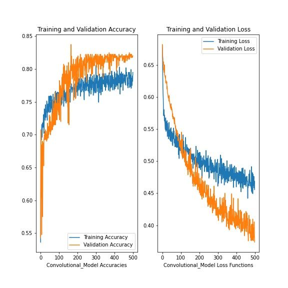
2 Data set                                                                                                              3

3 Methodology                                                                                                           4
  3.1 The data split . . . . . . .     .   .   .   .   .   .   .   .   .   .   .   .   .   .   .   .   .   .   .   .    4
  3.2 Data preprocessing . . . .       .   .   .   .   .   .   .   .   .   .   .   .   .   .   .   .   .   .   .   .    4
  3.3 Artificial Neural Networks       .   .   .   .   .   .   .   .   .   .   .   .   .   .   .   .   .   .   .   .    5
  3.4 Training and Evaluation .        .   .   .   .   .   .   .   .   .   .   .   .   .   .   .   .   .   .   .   .    8

4 Results and Discussion                                                                                                8

5 Conclusion                                                                                                           10

1     Introduction
    Machine Learning (ML) is defined as the study of algorithms that improve
their performances over given tasks when trained using input data. While
the field itself has existed for more than half a century, it is only in the
last 15 years that ML algorithms have begun to garner more attention from
researchers and companies that do work in other fields, as their performances
(measured by both the accuracies, and the real time necessary to train and
then to implement the algorithms) have improved enough to become relevant
and useful for many tasks [1].
   While many subfields of ML, such as Natural Language Processing, au-
tonomous driving and speech synthesis, have seen important breakthroughs
in the last few years, it is the study of image classification that has been most
impacted by the development of Deep Learning, more specifically the realiza-
tion that models called Convolutional Neural Networks allowed for greater
accuracies and for lower costs in labeling the data than ever before [2]. Com-
bined with the increasing data set sizes and the creation of better CPUs that
allowed for faster computation [3], Deep Learning algorithms have become
the mainstay of top-level ML research in this subject.
   Therefore, in recent times, neural networks have been one of the most
useful tools for astronomers in trying to recognize and classify many types
of objects in our solar system, as the field has become much more data-
rich. For instance, radio recordings have been successfully used to detect and
extract samples of meteors entering the Earth’s atmosphere [4]. Direct image
recognition has also been successful in identifying stars, galaxies and quasars
[5]. Because comets and asteroids, together named Near Earth Objects, can

                                           2
pose a serious threat to our planet [6], while also being useful case studies
for the development of our understanding of the solar system, it is important
that we apply the same proven methods to automatically detect asteroid
trails.
2 Data set
Our data set was made up of 2000 images, out of which 1036 contained
asteroid trails, while 964 did not. While some of these photos were obtained
from the Zooniverse site itself, most of them were offered by Sandor Kruk,
researcher working at ESA.
Figure 1: Asteroid trails
The sizes of the unprocessed images varied. Many of them had sizes be-
tween 1040-1060x1050-1070 px, while others had sizes ranging from 400-
800x400-800 px. These images were all almost square (with small differences
between their lengths and widths). An example of an image containing an
asteroid trail (on the bottom-left side) is provided in Figure 1, with a size of
1053x1059 px. Another example, of an image containing no asteroid trails,
is provided in Figure 2, with a size of 797x811 px.
As seen in Figure 1, some of the pictures taken were imperfect, as the
process of taking them was not uniform. However, the presence of the white
pixels and the fact that the images are not perfect rectangles were factors
that could be mitigated easily by reshaping the images and normalizing the
pixel values.
3Figure 2: No asteroid trails
3 Methodology
The sequence of steps taken in order to train and evaluate the models con-
sisted of splitting the images into training and validation sets, preprocessing
and augmenting the dataset, building and training multiple Convolutional
Neural Networks in Python, selecting the ones that performed best on the
training set and evaluating them on the validation set.
3.1 The data split
We decided to split the data into two separate sets (training and valida-
tion), using the recommended 80%-20% split.
This statistical split guaranteed us that the model would be properly
trained on a sufficiently large set of images, while also avoiding any pos-
sible over fitting problems, thus resulting in accuracies that would closely
match its performance on new, real-life data.
3.2 Data preprocessing
We used the ImageDataGenerator (IDG) class from Keras (running on top
of TensorFlow, in the programming language Python) in order to preprocess
the data set.
We utilized it to reshape the images to the target size of 256x256 px and
to change them to a grayscale representation, which allowed for fast training
4of the programs, while maintaining the relevant features of the photos. We
also normalized the image matrices by rescaling the values of the pixels to
be in the range [0, 1].
The ImageDataGenerator class created a batch of 32 augmented images
for every image that was introduced, by randomly rotating, zooming, shifting
and shearing the image (all within small, carefully-constructed ranges), thus
artificially outputting a larger training set of 51200 images that we could
train the model on.
Figure 3: Before using the IDG class
Figure 3 shows an example of a photo not containing asteroid trails, taken
from the Zooniverse site.
Meanwhile, Figure 4 shows an example of what 5 of the 32 artificially
generated photos could look like. All these photos were created from the
image displayed in Figure 3 by using transformations similar to the ones
described above. These generated photos were all zoomed in to some extent,
and thus they all mostly showed relatively different parts of the initial image,
however the actual transformations used smaller zooms than these, ensuring
that no asteroid trails were accidentally removed from the asteroid trail-
containing training set.
3.3 Artificial Neural Networks
The models we employed built upon the standard Artificial (Feedforward)
Neural Network (ANN) architecture used by Multilayer Perceptrons (shown
5Figure 4: After using the IDG class
in Figure 5), which consist of an input layer, followed by one or more hidden
layers that are tied together, one after another, for which the numbers in
the nodes are calculated as the values of the activation function of a linear
combination between the weights and bias terms and the values of the pre-
ceding layer, and by the output layer, whose activation function is typically
either the logistic function, or the rectified linear unit. The weights inherent
to these models are typically trained through an optimized version of the
process of gradient descent, generally using the backpropagation algorithm.
However, the models that performed best on the validation and test sets
were Convolutional Neural Networks (CNNs), versions of feedforward ANNs
that employed two pairs of Convolutional and Max Pooling layers. The
Convolutional layers first performed an operation called convolution on the
initial 256x256 array of pixels corresponding to the image, which consisted
of creating multiple new two-dimensional arrays through the dot product
between iterated sections of the image and carefully-selected 2x2 filters, thus
capturing the crucial features embedded in the pixel array. Then, the models
employed the Pooling layers, a form of dimensionality reduction which selects
only the maximum pixel value in each section of the image, thus making the
6Figure 5: Standard structure of a feedforward ANN
model more robust and cheaper to train (other versions of Pooling layers also
exist, such as Average Pooling, but Max Pooling is typically considered most
suitable for these types of problems). The models were completed by the
addition of one deep layer and the final output one, which used a sigmoid
activation function. In order to reduce overfitting problems, the models also
employed two Dropout layers.
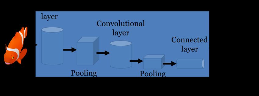
Figure 6 shows an example of what a CNN architecture looks like. The
increased use of Convolutional layers has been the key for the development
of Deep Learning as a very useful means of recognition and prediction [7],
especially for tasks involving computer vision [8], so it is no surprise that
models based upon it perform better than the general-use algorithms do.
7Figure 6: Standard structure of a CNN
3.4 Training and Evaluation
The process of training and evaluating the algorithms was done using of
Google Colab, a browser-based notebook environment similar to Jupyter
Notebook. This was done in order to benefit from the free availability of
Graphical Processing Units and Tensor Processing Units, which sped up the
learning process significantly.
The optimizer we used is called Stochastic Gradient Descent, and the mod-
els were trained for 500 epochs at the learning rate of 0.001. The models
aimed to minimize the Binary Crossentropy loss function on the training set.
Because the data sets were balanced, the models were compared based on
the accuracies they displayed on the validation sets.
4 Results and Discussion
The best models obtained an accuracy of 82% on the validation set, with a
Binary Crossentropy loss function of 0.3893. Figure 7 shows a plotting of the
accuracies and loss functions that the model obtained over the 500 epochs.
As can be seen from the confusion matrices in Figure 8, the precision of
the predictions is 77.45%, while the recall is 91.74%, for an overall F1 score
of 0.84.
Since the neural network’s accuracies on the validation set were similar to
and in some cases even exceeded those on the training set, there appears to
be almost no sign of over fitting, which means that carefully increasing its
depth would possibly result in even better results. However, this must be
8Figure 7: Plot of the model’s performance over time
balanced out with the fact that a large model would contain more than 40
million parameters and would thus be very hard to properly train. It also
means that increasing the size of the training data set, whether through the
capture of more images or through methods of synthetic data generation,
would probably not have improved the accuracy as much.
While the overall performance of the model was good, the relatively high
difference between its recall and its precision made the F1 score greater than
the accuracy, which showed that the model predicts that images contain
asteroid trails far too often.
The biggest problem the model faced was the relative subtlety of the as-
9Figure 8: Confusion matrices on the validation set
teroid trails in the images. They were mostly straight lines of a small width,
and such simple shapes were not as easily recognized by deep Convolutional
Neural Networks as more complex ones. On the other hand, one of their
built-in advantages was the ability to add augmented data in the training
sets with minimal additional computational cost, which is not the case with
other classifiers, such as Support Vector Machines.
5 Conclusion
Based on the resulting data, Deep Learning models using convolutional
layers, trained on an artificially generated training set of 51200 images, per-
formed adequately in classifying images of asteroid trails in space photos,
identifying them with accuracies of above 80% on the validation set.
There are several ideas and techniques which could improve the perfor-
mance of future models on similar tasks. For instance, utilizing large batches
of images of the same size and of a square shape could help avoid any reshape-
induced problems. Properly identifying and removing the large stars present
in the photos could eliminate much of the noise in the images and thus allow
the algorithms to learn how to identify asteroid trails faster. Using vary-
ing dilation rates for the convolutional kernels and implementing Average
Pooling layers instead of Max Pooling ones should also be considered.
Different architectures or types of models could also provide a starting
point for avoiding the issues that the CNNs faced. Combining the neu-
10ral network architecture with the kernel method, more commonly seen in
Support Vector Machines, has recently achieved outstanding results on the
CIFAR-10 dataset [9], and similar models could benefit from combining the
advantages of SVM-like methods (such as identifying simpler shapes) with
those of Artificial Neural Networks.
The continued development of Machine Learning algorithms bodes well for
the fields of Astronomy and Astrophysics. While ML remains under utilized
at the moment, models such as ours show that Deep Learning has great
applicability in these areas.
References
[1] Junfei Qiu, Qihui Wu, Guoru Ding, Yuhua Xu, and Shuo Feng. A sur-
vey of machine learning for big data processing. EURASIP Journal on
Advances in Signal Processing, 2016(1):67, 2016.
[2] Rikiya Yamashita, Mizuho Nishio, Richard Kinh Gian Do, and Kaori
Togashi. Convolutional neural networks: an overview and application in
radiology. Insights into imaging, 9(4):611–629, 2018.
[3] Noel Lopes and Bernardete Ribeiro. Towards adaptive learning with im-
proved convergence of deep belief networks on graphics processing units.
Pattern recognition, 47(1):114–127, 2014.
[4] VS Roman and Cătălin Buiu. Automatic detection of meteors using
artificial neural networks. In Proceedings of the International Meteor
Conference, Giron, France, pages 18–21, 2014.
[5] Ana Martinazzo, Mateus Espadoto, and Nina ST Hirata. Self-
supervised learning for astronomical image classification. arXiv preprint
arXiv:2004.11336, 2020.
[6] Harry Atkinson. Risks to the earth from impacts of asteroids and comets.
europhysics news, 32(4):126–129, 2001.
[7] Ian Goodfellow, Yoshua Bengio, Aaron Courville, and Yoshua Bengio.
Deep learning, volume 1. MIT press Cambridge, 2016.
11[8] Ian J Goodfellow, Yaroslav Bulatov, Julian Ibarz, Sacha Arnoud, and
Vinay Shet. Multi-digit number recognition from street view imagery us-
ing deep convolutional neural networks. arXiv preprint arXiv:1312.6082,
2013.
[9] Vaishaal Shankar, Alex Fang, Wenshuo Guo, Sara Fridovich-Keil, Ludwig
Schmidt, Jonathan Ragan-Kelley, and Benjamin Recht. Neural kernels
without tangents. arXiv preprint arXiv:2003.02237, 2020.
12You can also read