Digital Commons@Georgia Southern - Georgia Southern University - Digital ...
←
→
Page content transcription
If your browser does not render page correctly, please read the page content below
Georgia Southern University
                                                  Digital Commons@Georgia Southern

Honors College Theses

2021

Modeling the Stock Market Through Game Theory
Kylie Hannafey
Georgia Southern University

Follow this and additional works at: https://digitalcommons.georgiasouthern.edu/honors-theses

   Part of the Business Analytics Commons, Data Science Commons, and the Other Applied
Mathematics Commons

Recommended Citation
Hannafey, Kylie, "Modeling the Stock Market Through Game Theory" (2021). Honors College Theses. 590.
https://digitalcommons.georgiasouthern.edu/honors-theses/590

This thesis (open access) is brought to you for free and open access by Digital Commons@Georgia Southern. It
has been accepted for inclusion in Honors College Theses by an authorized administrator of Digital
Commons@Georgia Southern. For more information, please contact digitalcommons@georgiasouthern.edu.
MODELING THE STOCK MARKET THROUGH GAME THEORY

   An Honors Thesis submitted in partial fulfillment of the requirements for Honors in
                               Mathematical Science.

                                            by

                                   KYLIE HANNAFEY

                           Under the mentorship of Hua Wang

                                       ABSTRACT

Game Theory is used on many occasions to help us understand interactions between decision-
makers. The famous Nash equilibrium is a steady state in a model that shows the interaction
of different players, in which no player can do better by choosing a different action if the
actions of the other players do not change. These two concepts can be applied to numerous
situations that vary in types of players, but for our research, we are focusing on businesses
in the stock market. The main objective is to use Game Theory to analyze data collected
from the stock market, model our findings, predict decisions made by businesses, and un-
derstand what scenarios will produce a stable stock market. In particular, we will provide
a thorough analysis of the stock market behavior between the three leading competitors
in technology. We will first use statistical models to analyze and report data collected on
Apple, Microsoft, and Google from the stock market. To begin, we will use the website
Nasdaq, a detailed online record of the stock market, to record the daily price of stock and
share volume for each company. Then, we will use Excel to statistically analyze and model
our findings. As a result, we should be able to evaluate the stability of the stock market and
discuss the relationships between our companies. More specifically, we expect to find the
impact changes in the stock market have on each business and predict the behavior, or the
“best next move,” they should have.
                                Thesis Mentor:
                                                                                    Hua Wang

                            Honors Director:
                                                                          Dr. Steven Engel

                                       May 2021
                                 Mathematical Science
                               University Honors Program
                              Georgia Southern University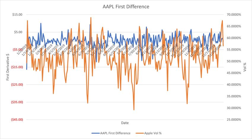
c 2021

KYLIE HANNAFEY

All Rights Reserved
2

                                ACKNOWLEDGMENTS

I wish to acknowledge my family, friends and outstanding professors at Georgia Southern.

Specifically, I would like to thank Dr. Hua Wang for all his help.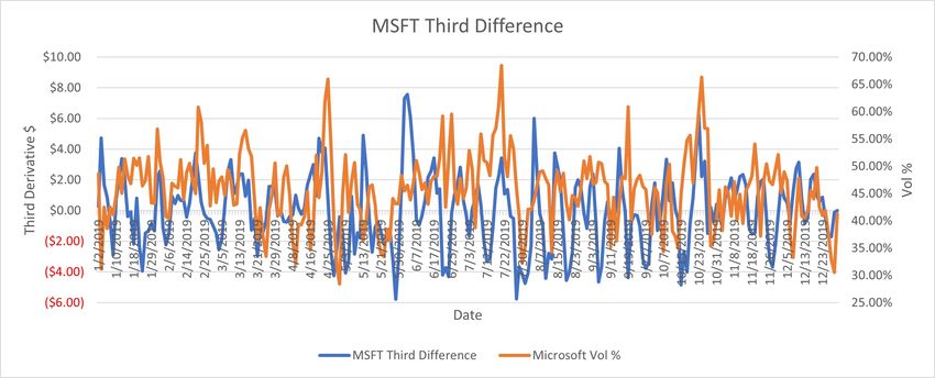
TABLE OF CONTENTS

                                                                                          Page

ACKNOWLEDGMENTS . . . . . . . . . . . . . . . . . . . . . . . . . . . . . .                 2

LIST OF TABLES       . . . . . . . . . . . . . . . . . . . . . . . . . . . . . . . . .      5

LIST OF FIGURES . . . . . . . . . . . . . . . . . . . . . . . . . . . . . . . . .           6

CHAPTER

       1   Introduction . . . . . . . . . . . . . . . . . . . . . . . . . . . . . . .       8

             1.1   Financial stability    . . . . . . . . . . . . . . . . . . . . . . .     8

             1.2   Game Theory and Nash Equilibrium . . . . . . . . . . . . . .             9

                1.2.1 Background . . . . . . . . . . . . . . . . . . . . . . . . .          9

                1.2.2 Formal definitions . . . . . . . . . . . . . . . . . . . . . .       10

                1.2.3 A first example     . . . . . . . . . . . . . . . . . . . . . . .    10

                1.2.4 A Second Example        . . . . . . . . . . . . . . . . . . . . .    11

             1.3   Cournot and Bertrand Game Theory Models . . . . . . . . . .             12

                1.3.1 Cournot’s model . . . . . . . . . . . . . . . . . . . . . . .        12

                1.3.2 Bertrand’s model      . . . . . . . . . . . . . . . . . . . . . .    13

       2   Data collection and analysis     . . . . . . . . . . . . . . . . . . . . . .    15

             2.1   Introduction     . . . . . . . . . . . . . . . . . . . . . . . . . .    15

             2.2   Collection     . . . . . . . . . . . . . . . . . . . . . . . . . . .    15

             2.3   Normalization      . . . . . . . . . . . . . . . . . . . . . . . . .    17

                                             3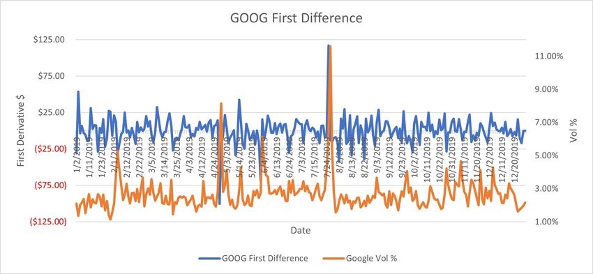
3   Data analysis for Game Theory model . . . . . . . . . . . . . . . . .         21

             3.1   Price data sets   . . . . . . . . . . . . . . . . . . . . . . . . .   21

             3.2   Volume data sets . . . . . . . . . . . . . . . . . . . . . . . .      24

             3.3   Relating price and volume data sets     . . . . . . . . . . . . . .   25

       4   Further directions and concluding remarks . . . . . . . . . . . . . . .       29

REFERENCES . . . . . . . . . . . . . . . . . . . . . . . . . . . . . . . . . . .         33

                                            4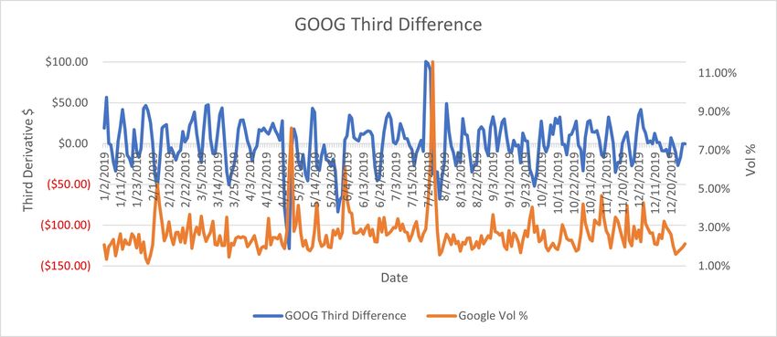
LIST OF TABLES

Table                                                                                     Page

        2.1   Apple . . . . . . . . . . . . . . . . . . . . . . . . . . . . . . . . . .    15

        2.2   Microsoft . . . . . . . . . . . . . . . . . . . . . . . . . . . . . . . .    16

        2.3   Google . . . . . . . . . . . . . . . . . . . . . . . . . . . . . . . . .     16

        2.4   Hourly Data . . . . . . . . . . . . . . . . . . . . . . . . . . . . . . .    16

        2.5   Multi-row table . . . . . . . . . . . . . . . . . . . . . . . . . . . . .    20

                                              5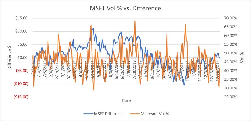
LIST OF FIGURES

Figure                                                                                 Page

     1.1   Inverse Demand Function from [5] . . . . . . . . . . . . . . . . . . .       13

     3.1   Apple (AAPL) Stock Price . . . . . . . . . . . . . . . . . . . . . . .       21

     3.2   Microsoft (MSFT) Stock Price . . . . . . . . . . . . . . . . . . . . .       21

     3.3   Google (GOOG) Stock Price . . . . . . . . . . . . . . . . . . . . . .        22

     3.4   AAPL Normalized Price     . . . . . . . . . . . . . . . . . . . . . . . .    22

     3.5   MSFT Normalized Price     . . . . . . . . . . . . . . . . . . . . . . . .    23

     3.6   GOOG Normalized Price . . . . . . . . . . . . . . . . . . . . . . . .        23

     3.7   AAPL Volume Percentage      . . . . . . . . . . . . . . . . . . . . . . .    24

     3.8   MSFT Volume Percentage      . . . . . . . . . . . . . . . . . . . . . . .    24

     3.9   GOOG Volume Percentage . . . . . . . . . . . . . . . . . . . . . . .         25

    3.10   AAPL Stock Price and Volume Percentage . . . . . . . . . . . . . . .         25

    3.11   MSFT Stock Price and Volume Percentage . . . . . . . . . . . . . . .         26

    3.12   GOOG Stock Price and Volume Percentage        . . . . . . . . . . . . . .    26

    3.13   AAPL Volume Percentage vs Difference . . . . . . . . . . . . . . . .         27

    3.14   MSFT Volume Percentage vs Difference . . . . . . . . . . . . . . . .         28

    3.15   GOOG Volume Percentage vs Difference . . . . . . . . . . . . . . . .         28

     4.1   AAPL First Difference Vector    . . . . . . . . . . . . . . . . . . . . .    29

                                          6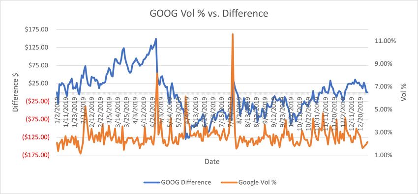
4.2   MSFT First Difference Vector   . . . . . . . . . . . . . . . . . . . . .     29

4.3   GOOG First Difference Vector . . . . . . . . . . . . . . . . . . . . .       30

4.4   AAPL Third Difference Vector . . . . . . . . . . . . . . . . . . . . .       30

4.5   MSFT Third Difference Vector . . . . . . . . . . . . . . . . . . . . .       31

4.6   GOOG Third Difference Vector       . . . . . . . . . . . . . . . . . . . .   31

                                     7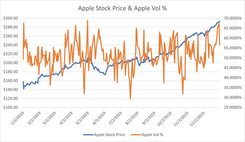
8

                                          CHAPTER 1
                                       INTRODUCTION

The majority of the theoretical background for this thesis can be found in [5].

                                 1.1   F INANCIAL STABILITY

Financial stability can be defined as such: “A financial system is in a range of stability
whenever it is capable of facilitating (rather than impeding) the performance of an econ-
omy, and of dissipating financial imbalances that arise endogenously or as a result of signif-
icant adverse and unanticipated events” [8]. Now let us unpack that definition. First of all,
“the stock market is an institution that connects potential buyers and sellers of companies’
stocks” [3]. The stock market is essentially a business. Using our definition of financial
stability, a business is considered financially stable if it is efficient with its resources, prof-
iting, making smart investments, and increasing in wealth. Essentially, a business must be
successful to improve the performance of an economy. In addition, the system must be able
to handle financial imbalances that occur due to internal issues or as a result of external,
unanticipated events. For a business in the stock market, this means if they made poor
investment choices or another business they have competition with does something, they
must be able to make the best next move to overcome the obstacle and stay in the game.
Game Theory strategy will help businesses in the stock market achieve financial stability.
Players in the game are making decisions that are in their best interest while also taking
into account what the other players are possibly doing. A player wants to succeed, but also
wants to survive, which is essentially what our definition of financial stability implies.
9
1.2 G AME T HEORY AND NASH E QUILIBRIUM
1.2.1 BACKGROUND
In the 1920s, Emile Borel and John Von Neumann developed Game Theory, which aims
to help us understand interactions between decision-makers [5]. It is formally defined as
the study of mathematical models of strategic interactions among rational decision-makers.
Von Neumann described two types of games: “In the first type, rule-based games, players
interact according to specified ‘rules of engagement’. In the second type, freewheeling
games, players interact without any external constraints” [2]. Business, specifically the
stock market, is a combination of these two types of games.
Game theory is very versatile and can be applied to a variety of situations. According
to Franklin Allen, “game theory has provided a methodology that has led to insights into
many previously unexplained phenomena by allowing asymmetric information and strate-
gic information to be incorporated in the analysis” [1]. The most common uses of game
theory include economic theory, political science, and psychology.
An important feature of game theory is the Nash equilibrium. The Nash equilibrium
was developed by the famous game theorist John Nash. He showed that “in any finite
game (i.e., a game in which the number of players n and the strategy sets Si , ..., S are
all finite) there exists at least one Nash equilibrium” [4]. A Nash equilibrium is a steady
state in a model in which no player can do better by choosing a different action if the
actions of the other players do not change [5]. Essentially, a Nash equilibrium is the best
response a player can make to any of the other players’ actions. There are also cases of
multiple Nash equilibria: “McLennan shows that standard normal-form games can have
enormous numbers of equilibria” [7]. An example of such a case is shown below in A
Second Example.10
1.2.2 F ORMAL DEFINITIONS
Definition 1. Game Theory: The study of mathematical models of strategic interactions
among rational decision-makers.
Definition 2. Payoff Function: It essentially ranks each action according to its preferability.
It is another way to represent the preferences of players.
Definition 3. Best Response Function: The best action a player can make given the other
player’s action. It is the action that will yield player A the highest payoff value given player
B’s action.
Definition 4. Nash Equilibrium: A steady state in a model in which no player can do better
by choosing a different action if the actions of the other players do not change.
1.2.3 A FIRST EXAMPLE
The best game theory example is the Prisoner’s Dilemma. In this problem, there are two
prisoners and they each have two choices: stay quiet or confess. If they both stay quiet, then
they each get one year of jail. If one stays quiet, but the other confesses, then the person
who confessed gets 0 years and the person who stayed quiet gets 4 years and vice-versa.
Finally, if they both confess, then they both get 3 years of jail time. This is modeled in the
table below.
Prisoner 2
Quiet Confess
Quiet (1, 1) (4, 0)
Prisoner 1
Confess (0, 4) (3, 3)
The number of years spent in jail can be represented using payoff values. Payoff
values essentially rank each action according to its preferability. In this case, each action11
will be ranked from 0-3, with 3 meaning it is the most preferred action. So, four years in
jail would have a payoff value of 0. Three years in jail would have a payoff value of 1. One
year would have a payoff value of 2. Finally, zero years in jail would have a payoff value
of 3. This can be modeled in the table below. We also can mark a player’s best response to
each action of the other player using “*”. The box that ends up with two “*” is the Nash
equilibrium.
Quiet Confess
Quiet (2, 2) (0, 3∗ )
Confess (3∗ , 0) (1∗ , 1∗ )
From looking at this table, one can see that the Nash equilibrium is (Confess, Confess).
This is because, given that Prisoner 2 chooses Confess, Prisoner 1 is better off choosing
Confess rather than Quiet (looking at the first entries in the right column, Quiet yields
Prisoner 1 and payoff value of 0 and Confess yields them a payoff value of 1), and vice
versa. Given that Prisoner 1 chooses Confess, Prisoner 2 is better off choosing Confess
rather than Quiet (looking at the second entries in the second row, Quiet yields Prisoner 2
a payoff value of 0 and Confess yields them a payoff value of 1).
1.2.4 A S ECOND E XAMPLE
Another great game theory example is the Battle of the Sexes. In this problem, there is a
man and woman trying to decide where to go out for the night, either to a football game or a
ballet performance. They would both rather spend the night together than apart. However,
the woman prefers they both go to the ballet performance, but the man prefers they both go
to the football game [6]. Their preferences can be modeled below.
Football Ballet
Football (2∗ , 1∗ ) (0, 0)
Ballet (0, 0) (1∗ , 2∗ )12
In this problem, (Football, Football) and (Ballet, Ballet) are Nash equilibria [6].
1.3 C OURNOT AND B ERTRAND G AME T HEORY M ODELS
1.3.1 C OURNOT ’ S MODEL
In general, there is a single good being produced by n firms. The cost for firm i to produce
qi units of the good is Ci (qi ), where Ci is increasing. Also, the firms’ total output is Q and
the market price is P (Q) (P is a decreasing function when positive) [5].
Cournot’s oligopoly game consists of firms as the players and the actions for each firm
are its possible outputs. The preferences of each firm are represented by its profit (1.1) [5].
πi (q1 , ..., qn ) = qi P (q1 + ... + qn ) − Ci (qi ). (1.1)
Example 1.1. We can look at an example from [5]. Suppose there are two firms with the
same cost function: Ci (qi ) = cqi for all qi . The inverse demand function is given by (1.2).
α − Q if Q ≤ α
P (Q) = (1.2)
0
if Q > α
where α > 0 and c ≥ 0 are constants. We can see the graph of the inverse demand
function in Figure 1.1.13
↑
P (Q)
α
0 α Q→
Figure 1.1: Inverse Demand Function from [5]
1.3.2 B ERTRAND ’ S MODEL
In general, there is a single good being produced by n firms. The cost for firm i to produce
qi units of the good is Ci (qi ), where Ci is increasing. Also, p is the price and demand is
D(p). If all the firms set different prices, then consumers will buy the goods at the lowest
price. Firms also only produce what is demanded [5].
Bertrand’s oligopoly game consists of firms as the players and the actions for each
firm are the possible prices. The preferences of each firm are represented by its profit (1.3)
[5].
p1 D(p1 ) − C1 (D(p1 )) if p1 < p2
πi (p1 , p2 ) = 1/2p1 D(p1 ) − C1 (1/2D(p1 )) if p1 = p2 (1.3)
0
if p1 > p2
Example 1.2. We can look at an example from [5]. Suppose there are two firms with the
same cost function: Ci (qi ) = cqi for i = 1, 2. The demand function is D(p) = α − p for
p ≤ α and D(p) = 0 for p > α, and c < α. To find the Nash equilibria of the game, we
must find the firms’ best response functions. Following [5], “we can look at firm i’s payoff14 as a function of its price pi for various values of the price pj of firm j.” One can see the graphs of each payoff function in Figure 63.1 in [5].
15

                                              CHAPTER 2
                          DATA COLLECTION AND ANALYSIS

                                        2.1     I NTRODUCTION

Our data will be collected from an online stock market database called Nasdaq and we will
record the stock price for each business, and the share volume as well, to obtain payoff
values.
     Stock price is the price at which each stock is sold. We chose to record it because
we believe it will give us a great deal of information as to how the company is doing on
a surface level. Share volume is the number of shares traded in a given time period. We
chose to record it because share volume will give us more insight into how the company
is doing on a deeper level. Share volume measures the effort behind movement in stock
prices. It shows how many investors, stockholders, etc. were involved in that move.

                                         2.2      C OLLECTION

Here, we show off some exemplary data of the stock prices and volume of shares of Apple,
Microsoft, and Google, over the month of March 2020, in Tables 2.1, 2.2, 2.3.

                             3/5           3/10         3/16         3/20          3/25         3/30

           Stock Price     292.92        285.34        242.21       229.24        245.52       254.81

          Vol of Shares    46,893,220     71,322,520   80,605,870   100,423,300   75,900,510   41,994,110

            Variation       8.14          17.07        19.08        23.83         13.95         6.12

                                          Table 2.1: Apple
16
Data type\Date 3/5 3/10 3/16 3/20 3/25 3/30
Stock Price 166.27 160.92 135.42 137.35 146.92 160.23
Volume of Shares 47,817,250 65,354,390 87,905,870 84,866,220 75,638,220 63,420,330
Variation 5.18 8.45 14.35 11.24 9.89 10.59
Table 2.2: Microsoft
Data type\Date 3/5 3/10 3/16 3/20 3/25 3/30
Stock Price 1319.04 1280.39 1084.33 1072.32 1102.49 1146.82
Volume of Shares 2,561,288 2,611,373 4,252,365 3,601,750 4,081,528 2,574,061
Variation 53.81 62.38 77.83 78.50 62.89 55.15
Table 2.3: Google
As an example of more detailed changes of the market, Table 2.4 shows the data for
the same three stocks at an hourly rate on April 7 2020.
Stock\Hour 8am 9am 10am 11am 12pm 1pm 2pm 3pm 4pm 5pm
Apple 268.30 270.10 269.43 264.25 265.96 266.04 263.13 260.17 259.43 258.45
MSFT 169.36 169.81 167.95 165.50 166.33 167.30 166.34 164.48 163.46 163.08
GOOGL 1219.09 1220.50 1214.18 1191.63 1198.98 1207.19 1202.69 1196.55 1186.51 1184.00
Table 2.4: Hourly Data17
2.3 N ORMALIZATION
To analyze the behavior of these different but related stocks, we take data similar to the
above, but from previous years. As the goal is to observe the behavior of these three stocks
and their impact upon each other, we often normalize our collected data.
Over the same period of time, we use pA , pM and pG to denote the vectors of prices
over time. For example, from Tables 2.1, 2.2, 2.3 we have
pA = h292.92, 285.34, 242.21, 229.24, 245.52, 254.81i,
pM = h166.27, 160.92, 135.42, 137.35, 146.92, 160.23i,
and
pG = h1319.04, 1280.39, 1084.33, 1072.32, 1102.49, 1146.82i.
For such a “price vector”, p = hp1 , p2 , . . . , pn i, let
n
X
p= pi /n
i=1
and the “normalized price vector” be
p1 p2 pn
P = , ,..., .
p p p
Taking the above data as an example, we have
292.92 285.34 242.21 229.24 245.52 254.81
PA = , , , , ,
258.34 258.34 258.34 258.34 258.34 258.34
= h1.1339, 1.1045, 0.9376, 0.8874, 0.9504, 0.9863i .
166.27 160.92 135.42 137.35 146.92 160.23
PM = , , , , ,
151.19 151.19 151.19 151.19 151.19 151.19
= h1.0997, 1.0644, 0.8957, 0.9085, 0.9718, 1.0598i .18
1319.04 1280.39 1084.33 1072.32 1102.49 1146.82
PG = , , , , ,
1167.57 1167.57 1167.57 1167.57 1167.57 1167.57
= h1.1297, 1.0966, 0.9287, 0.9184, 0.9443, 0.9822i .
As for the “volume vectors” v A , v M and v G , we let
(V α ) = (v α ) /v
for α = A, M, G respectively, where
v i = (v A )i + (v M )i + (v G )i
for i = 1, 2, . . . , n.
With Tables 2.1, 2.2, 2.3 we now have
v A = h46, 893, 220, 71, 322, 520, 80, 605, 870, 100, 423, 300, 75, 900, 510, 41, 994, 110i,
v M = h47, 817, 250, 65, 354, 390, 87, 905, 870, 84, 866, 220, 75, 638, 220, 63, 420, 330i,
v G = h2, 561, 288, 2, 611, 373, 4, 252, 365, 3, 601, 750, 4, 081, 528, 2, 574, 061i.
And
v = hv 1 , . . . , v n i
= h97271758, 139288283, 172764105, 188891270, 155620258, 107988501i
So,
V A = h48.2085%, 51.2050%, 46.6566%, 53.1646%, 48.7729%, 38.8876%i
V M = h49.1584%, 46.9202%, 50.8820%, 44.9286%, 48.6044%, 58.7288%i19
V G = h2.6331%, 1.8748%, 2.4614%, 1.9068%, 2.6227%, 2.3836%i
Take f α for the variation data, define f accordingly (similar to p) and let
f
Rα =
p
for α = A, M, G. This is our “risk” factor. Again, from Tables 2.1, 2.2, 2.3, we have
n
X
f= fi /n
i=1
So,
f A = 14.6983
f M = 9.95
f G = 65.0933
This means our risk factors for α = A, M, G are
14.6983
RA = = 0.056895
258.34
9.95
RM = = 0.065811
151.19
65.0933
RG = = 0.055751
1167.57
We may summarize our data in the following Table 2.5.20
Table 2.5: Multi-row table
PA 1.1339 1.1045 0.9376 0.8874 0.9504 0.9863
Apple VA 48.2085% 51.2050% 46.6566% 53.1646% 48.7729% 38.8876%
RA 0.056895
PM 1.0997 1.0644 0.8957 0.9085 0.9718 1.0598
Microsoft VM 49.1584% 46.9202% 50.8820% 44.9286% 48.6044% 58.7288%
RM 0.065811
PG 1.1297 1.0966 0.9287 0.9184 0.9443 0.9822
Google VG 2.6331% 1.8748% 2.4614% 1.9068% 2.6227% 2.3836%
RG 0.05575121
CHAPTER 3
DATA ANALYSIS FOR GAME THEORY MODEL
In this chapter we show how the practical data is handled.
3.1 P RICE DATA SETS
First, we recorded the average stock price, the daily high and low stock price, and share
volume for Apple, Microsoft, and Google during the year 2019. From there, we graphed
the average stock price over 2019 for each company (see Figures 3.1, 3.2, 3.3 below).
Figure 3.1: Apple (AAPL) Stock Price
Figure 3.2: Microsoft (MSFT) Stock Price22
Figure 3.3: Google (GOOG) Stock Price
Since the general stock prices have always been fluctuating, this data should be “nor-
malized” before they can more precisely reflect the changes on the market. For this purpose,
we calculated the normalized stock prices for each company by taking the daily stock price
and dividing it by the yearly average stock price. The graphs for each can be seen below in
Figures 3.4, 3.5, 3.6.
Figure 3.4: AAPL Normalized Price23 Figure 3.5: MSFT Normalized Price Figure 3.6: GOOG Normalized Price
24

                              3.2   VOLUME DATA SETS

Similarly, the volume of stocks has been constantly growing. Hence, we need to normalize
our gathered data accordingly. We calculated Apple’s volume percentage by adding up
Apple, Microsoft, and Google’s share volume for each day, and dividing Apple’s daily
share volume by that sum. We used a similar method to also find Microsoft and Google’s
volume percentages. The graphs for the companies’ volume percentage over 2019 can be
found below.

                         Figure 3.7: AAPL Volume Percentage

                         Figure 3.8: MSFT Volume Percentage
25
Figure 3.9: GOOG Volume Percentage
3.3 R ELATING PRICE AND VOLUME DATA SETS
Then, to see if there was any correlation, we graphed the stock price and volume percentage
together, shown in Figures 3.10, 3.11, 3.12.
Figure 3.10: AAPL Stock Price and Volume Percentage26 Figure 3.11: MSFT Stock Price and Volume Percentage Figure 3.12: GOOG Stock Price and Volume Percentage
27
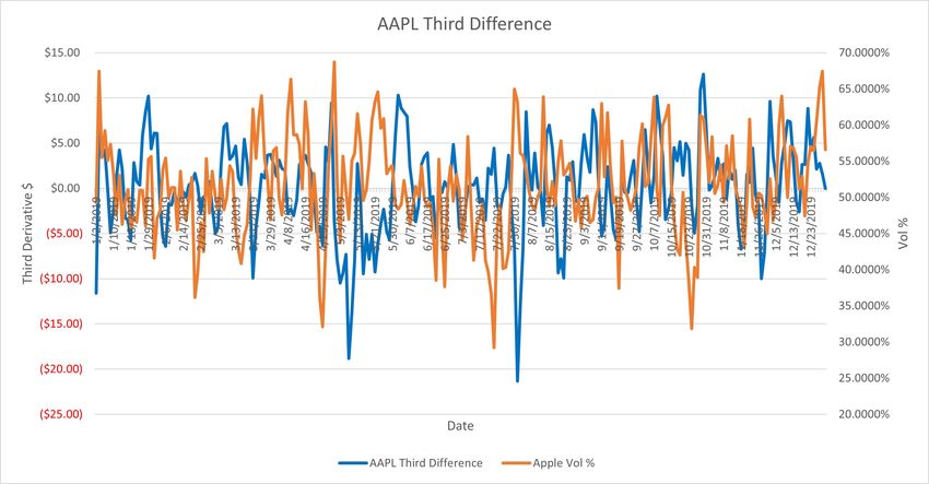
There was no discernible pattern in these figures, this is partly because of the ‘normal-
ized’ volume data and the generally increasing prices. Therefore, we developed a different
approach. We used Apple’s stock price data and graphed the 1/1/2019 point and 12/31/2019
point and made a straight line, corresponding to the underlying linear progression of the
price. By taking the difference of the original (normalized) price data and this new “line
data” (a new line with NEW stock prices labeled as “Apple Difference Prices”), a new
data set for AAPL price is obtained. We combined that graph with the volume percentage
graph. In doing so, there seemed to be more of a trend or pattern going on, as shown in
Figure 3.13.
Figure 3.13: AAPL Volume Percentage vs Difference
We did the same process with Microsoft and Google’s data which one can see in
Figures 3.14 and 3.15.28 Figure 3.14: MSFT Volume Percentage vs Difference Figure 3.15: GOOG Volume Percentage vs Difference
29
CHAPTER 4
FURTHER DIRECTIONS AND CONCLUDING REMARKS
While the Volume Percentage vs. Difference graphs did show more of a trend going on,
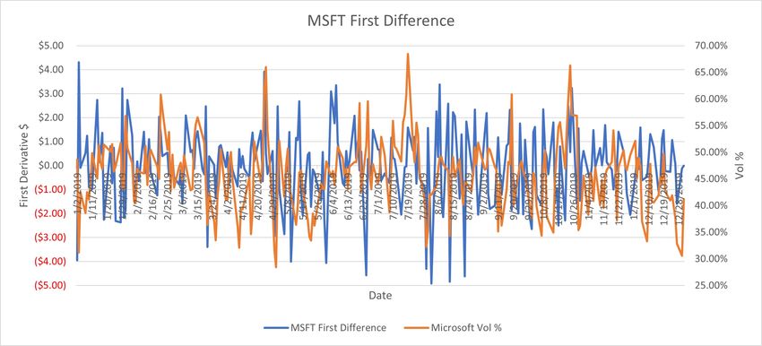
we wanted a more concrete pattern. So, we took the first (discrete) “derivative”, called the
difference vector, of our data. By this, we mean we subtracted the Day 2 difference by the
Day 1 difference and graphed it against the volume percentage (Figures 4.1, 4.2, 4.3).
Figure 4.1: AAPL First Difference Vector
Figure 4.2: MSFT First Difference Vector30
Figure 4.3: GOOG First Difference Vector
As you can see, the first difference vector either mirrors or correlates with the volume
percentage.
To further investigate, we found the third difference vector of our data. Meaning, we
subtracted the Day 4 difference by the Day 1 difference and graphed it against the volume
percentage (Figures 4.4, 4.5, 4.6).
Figure 4.4: AAPL Third Difference Vector31 Figure 4.5: MSFT Third Difference Vector Figure 4.6: GOOG Third Difference Vector
32

        Again, we found that the third difference vector either mirrors or correlates with the
volume percentage.
        In this thesis, we explored potential Game Theory models and data analysis approaches
for studying the stock market behavior. For future studies, one may work on combining the
two topics and find a game theory model that shows the Nash equilibrium of our collected
data.
33
REFERENCES
[1] Allen, Franklin and Stephen Morris. “Finance Applications of Game Theory.” Yale
University, 1998.
[2] Brandenburger, Adam M., and Barry J. Nalebuff. “The Right Game: Use Game Theory
to Shape Strategy.” Harvard Business Review, 1995.
[3] Fox, Merritt B., Lawrence R. Glosten and Gabriel V. Rautenberg. “The New Stock
Market: Sense and Nonsense.” Duke Law Journal, vol. 65, no. 2, 2015.
[4] Gibbons, Robert. “Game Theory for Applied Economists.” Princeton University
Press, 1992.
[5] Osborne, Martin J. “An Introduction to Game Theory.” Oxford University Press, 2000.
[6] Peters, Hans. “Game Theory: A Multi-Level Approach. Second Edition.” Springer
Texts in Business and Economics, 2015.
[7] Samuelson, Larry. “Game Theory in Economics and Beyond.” Journal of Economic
Perspectives, vol. 30, no. 4, 2016.
[8] Schinasi, Garry J. “Defining Financial Stability.” International Monetary Fund, No.
04/187, 2004.You can also read