The CASA software package - Dirk Petry (ESO), October 2010
←
→
Page content transcription
If your browser does not render page correctly, please read the page content below
The CASA software package
     Dirk Petry (ESO), October 2010

 Outline

 → What is CASA?                       - main features

 → Who develops CASA?                  - development team

 → What are the main requirements
   and how does CASA meet them?        - design and implementation

 → CASA status and release plans

 → How does CASA look and feel?        - installation and the typical analysis session

D. Petry, IRAM Interferometry School, Grenoble, October 2010                             1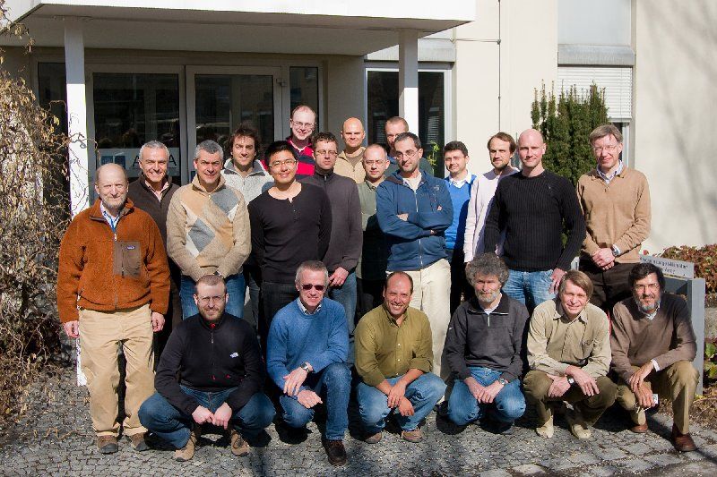
CASA main features

      - CASA = Common Astronomy Software Applications
      - Development started in the 90s as the next generation of AIPS
      - Refocussed in 2003 to be the ALMA/EVLA analysis package
      - Has the intention to be a general software package to reduce both
        interferometer and single-dish data
      - Internally consists of two parts:

                    User interface, higher-level analysis routines, viewers
                                      = casa non-core

                  General physical and astronomical utilities, infrastructure
                                       = casacore

      - Implements the “Measurement Equation” (Hamaker, Bregman & Sault 1996)
      - Internal data format is the “Measurement Set” (Kemball & Wieringa 2000)
      - 1.5 Million lines of code (mostly C++)
      - In public release under GNU Public License since December 2009

D. Petry, IRAM Interferometry School, Grenoble, October 2010                      2
CASA – development team
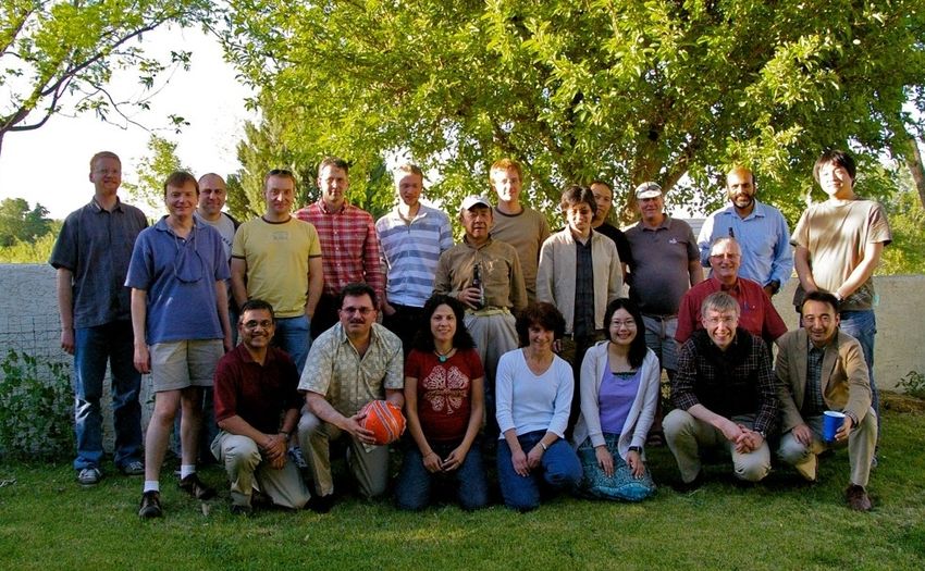
CASA Developers Meeting, NRAO, Socorro, May 2010
D. Petry, IRAM Interferometry School, Grenoble, October 2010 3CASA – development team
ESO ALMA Computing Group, February 2009
Since mid 2008, two CASA developers at ESO, since Sept. 2009 three
D. Petry, IRAM Interferometry School, Grenoble, October 2010 4CASA – development team
Originally only developed at NRAO (Socorro, NM), now
approx. 19 FTE developers are at work at
US (NRAO and others): 12
Japan (NAOJ): 3
Europe (ESO and others): 4
+ 1 CASA manager (NRAO Socorro) = Jeff Kern
+ 1 Project Scientist (NRAO Socorro) = Jürgen Ott
+ a few 5% FTEs at ASTRON, ATNF, and other places
Also involved:
ALMA Computing Managers = B. Glendenning (NRAO), G. Raffi, P. Ballester (ESO)
D. Petry, IRAM Interferometry School, Grenoble, October 2010 5CASA design and implementation Overall architecture: 1) A data structure 2) A set of data import/export facilities 3) A set of tools for data access, display, and editing 4) A set of tools for science analysis 5) A set of high-level analysis procedures (“tasks”) 6) A programmable command line interface with scripting 7) Documentation D. Petry, IRAM Interferometry School, Grenoble, October 2010 6
CASA design and implementation

Overall architecture:
1) A data structure
     Tables: Images, Caltables, and the Measurement Set (MS)
2) A set of data import/export facilities
     the so-called fillers: (ASDM, UVFITS, FITS-IDI, VLA archive) → MS, FITS → Image
3) A set of tools for data access, display, and editing
     tools to load/write data into/from casacore data types,
     Qt-based table browser, viewer, and (beta) x/y plotter, matplotlib-based x/y plotter
4) A set of tools for science analysis
     built around the Measurement Equation (developed in 1996),
    a toolkit for radio astronomical calibration, imaging, and simulation
5) A set of high-level analysis procedures (“tasks”)
     user-friendly implementations of the solutions for all common analysis problems
6) A programmable command line interface with scripting
     Python (augmented by IPython) gives a MATLAB-like interactive language
7) Documentation
     an extensive cookbook (500 pages) + documentation through help commands
    (help, ?, pdoc) + online help pages, See http://casa.nrao.edu/

D. Petry, IRAM Interferometry School, Grenoble, October 2010                                7
CASA design and implementation
Overall architecture:
1) A data structure
a) Tables: Images, Caltables, and the Measurement Set (MS)
2) A set of data import/export facilities
the so-called fillers: (ASDM, UVFITS, FITS-IDI, VLA archive) → MS, FITS → Image
3) A set of tools for data access, display, and editing
tools to load/write data into/from casacore data types,
Qt-based table browser, viewer, and (beta) x/y plotter, matplotlib-based x/y plotter
4) A set of tools for science analysis
b) built around the Measurement Equation (developed in 1996),
a toolkit for radio astronomical calibration, imaging, and simulation
5) A set of high-level analysis procedures (“tasks”)
user-friendly implementations of the solutions for all common analysis problems
6) A programmable command line interface with scripting
c) Python (augmented by IPython) gives a MATLAB-like interactive language
7) Documentation
an extensive cookbook (500 pages) + documentation through help commands
(help, ?, pdoc) + online help pages, See http://casa.nrao.edu/
D. Petry, IRAM Interferometry School, Grenoble, October 2010 8CASA design and implementation
CASA special features:
a) the Measurement Set (MS)
- developed by Cornwell, Kemball, & Wieringa between 1996 and 2000
- designed to store both interferometry (multi-dish) and single-dish data
- supports (in principle) any setup of radio telescopes
- supports description and processing of the data via the Measurement Equation
- fundamental storage mechanism: CASA Tables (inspired by MIRIAD)
- MS = table for radio telescope data (visibilities) + auxiliary sub-tables
D. Petry, IRAM Interferometry School, Grenoble, October 2010 9CASA design and implementation
The Measurement Set
MAIN none - - ANTENNA_ID ANTENNA ANTENNA_ID row number MAIN (ORBIT_ID) POLARIZATION POLARIZATION_ID row number DATA_DESCRIPTION none
FEED_ID FEED (PHASED_ARRAY_ID)
DATA_DESC_ID FREQ_OFFSET
PROCESSOR_ID POINTING
(PHASE_ID) SYSCAL
FIELD_ID
(PULSAR_GATE_ID)
WEATHER (SOURCE) SOURCE_ID explicit (DOPPLER) SPW_ID
FIELD (PULSAR_ID)
ARRAY_ID
OBSERVATION_ID FEED FEED_ID explicit MAIN ANTENNA_ID
STATE_ID FREQ_OFFSET SPW_ID
SYSCAL BEAM_ID
(PHASED_FEED_ID) (DOPPLER) DOPPLER_ID explicit SPW_ID SOURCE_ID
TRANSITION_ID
(FREQ_OFFSET) none - - ANTENNA_ID
FEED_ID DATA_DESCRIPTION DATA_DESC_ID row number MAIN SPW_ID
SPW_ID POLARIZATION_ID
(LAG_ID)
(SYSCAL) none - - ANTENNA_ID
PROCESSOR PROCESSOR_ID row number MAIN TYPE_ID
FEED_ID
SPW_ID MODE_ID
(PASS_ID)
POINTING none - - ANTENNA_ID FIELD FIELD_ID row number MAIN SOURCE_ID
POINTING_MODEL_ID (EPHEMERIS_ID)
OBSERVATION OBSERVATION_ID row number MAIN none
HISTORY
(WEATHER) none - - ANTENNA_ID
STATE STATE_ID row number MAIN none
HISTORY none - - OBSERVATION_ID
SPW SPW_ID row number DATA_DESCRIPTION (RECEIVER_ID)
OBJECT_ID
FEED (DOPPLER_ID)
FREQ_OFFSET (ASSOC_SPW_ID)
SOURCE
SYSCAL
FLAG_CMD none - - none
Legend: Level 1: Tables not referenced by other tables
[Table Name] [Key defined in this table] [key definition method] [referenced by] [referenced keys] Level 2: Tables referenced by level 1
(optional)
reference to table
outside the MS definition
Level 3: Tables referenced by level 2
V1, D.Petry, 13.2.09
D. Petry, IRAM Interferometry School, Grenoble, October 2010 10CASA design and implementation
CASA special features:
b) A toolkit for radio astronomical calibration, imaging, and simulation built around
the Measurement Equation (Hamaker, Bregman, & Sault 1996 + Sault, Hamaker, & Bregman 1996)
where
the vectors are: V = observed visibility = f(u, v), I = Image to be derived,
A = additive baseline-based error component
the matrices are: M = multiplicative, baseline-based error component
B = bandpass response
G = generalised electronic gain
D = polarisation leakage
E = antenna voltage pattern, i.e. primary beam effects
P = parallactic angle dependence
T = tropospheric effects
F = ionospheric Faraday rotation
S = mapping of I to the polarization basis of the observation
other variables and indices are:
l, m = image plane coordinates, i, j = telescope ID pairs = baseline, u, v = Fourier plane coordinates
D. Petry, IRAM Interferometry School, Grenoble, October 2010 11CASA design and implementation
CASA special features:
b) A toolkit for radio astronomical calibration, imaging, and simulation built around
the Measurement Equation (Hamaker, Bregman, & Sault 1996 + Sault, Hamaker, & Bregman 1996)
(continued)
Assuming, e.g., independence of the matrices from (l,m), the ME can be
solved for individual calibration components.
ideal visibility known from calibrator source
⇒ have set of linear equations.
The actual calculation of the component is then a χ2 minimization.
(For wide-field imaging the above assumption doesn't hold and the solution is
more complex but still possible.)
CASA contains a set of solvers for the different calibration components.
D. Petry, IRAM Interferometry School, Grenoble, October 2010 12CASA design and implementation
CASA special features:
b) A toolkit for radio astronomical calibration, imaging, and simulation (continued)
Imaging in CASA: Combinations of Major and Minor Cycle Algorithms
Imaging (Major Cycle):
1) Standard (no dir.-dep. effects, uv-grid sampling uses convolutional regridding)
2) with dir.-dep. effects:
a) W-term (image domain faceting, uv domain faceting, W projection)
b) PB correction (image domain, A projection)
c) Pointing Offset correction by phase gradient
d) Mosaicing (linear (separate) deconvolution,
joined deconv. of combined dirty images,
mosaicing by regridding all uv data onto one grid)
Deconvolution (Minor Cycle):
1) CLEAN (delta function model)
2) MS-CLEAN (blob model)
3) MSMFS CLEAN (model of blobs with polynomial spectrum)
4) MEM (maximum entropy method using prior image and delta function model)
see nice overview compiled by Urvashi Rau: https://safe.nrao.edu/wiki/bin/view/Software/AlgorithmList
D. Petry, IRAM Interferometry School, Grenoble, October 2010 13CASA design and implementation
CASA special features:
b) A toolkit for radio astronomical calibration, imaging, and simulation (continued)
A sophisticated radio-astronomical data simulator: simdata
- Create Measurement Sets of simulated data
(and for convenience: analyse the simulated MS to create simulated image)
- Input:
a) FITS image
b) “antenna list” file describing your interferometer (incl. site name)
sites: browsetable(os.getenv("CASAPATH").split(' ')[0]+"/data/geodetic/Observatories")
arrays: ls os.getenv("CASAPATH").split(' ')[0]+"/data/alma/simmos/"
c) observation setup parameters
(central direction, time, mosaicing, spectral, integration time, etc.)
d) corrupting effect parameters
(thermal noise from atmosphere and receiver)
- uses realistic site-dependent troposphere model
- knows about ALMA and EVLA receiver parameters
- phase noise and gain drift can be applied to the MS later via CASA tools
e) for convenience: clean task parameters for output image creation
D. Petry, IRAM Interferometry School, Grenoble, October 2010 14CASA design and implementation
CASA special features:
c) A programmable command line interface with scripting
Framework Architecture of 18 tools bound to Python (augmented by IPython)
at – atmosphere library
ms – Measurement Set utilities
mp – Measurement Set Plotting, e.g. data (amp/phase) versus other quantities
cb – Calibration utilities
cp – Calibration solution plotting utilities
im – Imaging utilities
ia – Image analysis utilities
fg – flagging utilities
tb – Table utilities (selection, extraction, etc.)
me – Measures utilities
tp – table plot
vp – voltage patterns
qa – Quanta utilities
cs – Coordinate system utilities
pl – matplotlib functionality
sd - ASAP = ATNF Spectral Analysis Package (single-dish analysis imported from ATNF)
sm - simulation
sl - spectral line tool (new in CASA 3.1!)
D. Petry, IRAM Interferometry School, Grenoble, October 2010 15CASA design and implementation
CASA special features:
c) A programmable command line interface with scripting
(continued)
Python (augmented by IPython)
Gives features such as
- tab completion
- autoparenthesis
- command line numbering
- access to OS, e.g.
Lines starting with ‘!’ go to the OS.
a = !ls *.py to capture the output of ‘ls *.py’.
!cmd $myvar expands Python var myvar for the shell.
- history
- execfile()
- comfortable help
D. Petry, IRAM Interferometry School, Grenoble, October 2010 16CASA design and implementation
CASA special features:
c) A programmable command line interface with scripting
(continued)
In addition to toolkit: high-level tasks for the standard user
tasks (implemented in Python) tools (implemented in C++)
e.g. the task importfits is based on the tool ia (image analysis):
#Python script
casalog.origin('importfits')
ia.fromfits(imagename,fitsimage,whichrep,whichhdu,zeroblanks,overwrite)
ia.close()
CASA 3.1 comes with 106 implemented tasks.
D. Petry, IRAM Interferometry School, Grenoble, October 2010 17CASA status
● Since Dec 2009 in public release under GPL = anybody can download,
no warranty (see http://casa.nrao.edu ),
limited support (help desk, needs registration)
● Tutorials for the user community regularly given
● The first public release was CASA 3.0.0 (Dec 2009), release 3.1.0 coming before Dec. 2010
● Development platforms: Linux (RHEL) + Mac OS X
● Supported platforms (binary distribution): RHEL, Fedora, openSuSE, Ubuntu, Mac OS X
● Code kept in svn repository at NRAO, Socorro
● Have approx. 4300 modules, 1.5E6 lines of code, 1E6 lines of comments
● The core functionality (casacore, also available at http://code.google.com/p/casacore/ )
is also used by other projects
● Hot topics:
- Support for High Performace Computing and Parallelisation
- Advanced Imaging: wide fields, continuum imaging over wide spectral ranges
- Interoperability: using CASA for other observatories and VLBI
D. Petry, IRAM Interferometry School, Grenoble, October 2010 18How does CASA look and feel?
flagging
A typical analysis session
Part 1: flagging and
calibration
D. Petry, IRAM Interferometry School, Grenoble, October 2010 19How does CASA look and feel?
A typical analysis session
Part 2: imaging and
image analysis imaging
image cube
numerical viewing,
analysis plotting
publication-ready plots and numerical results
D. Petry, IRAM Interferometry School, Grenoble, October 2010 20How does CASA look and feel?
Installation - CASA comes as a tgz-file for Linux or a dmg-file for Mac OS-X
Download latest version at
https://svn.cv.nrao.edu/casa/linux_distro
or
https://svn.cv.nrao.edu/casa/osx_distro
Linux:
Unpack tgz file in a location of your choice.
cd into the created casapy directory.
export PATH=$PWD:$PATH
Mac OS-X:
Open the CASA disk image file (if your browser does not do so automatically).
Drag the CASA application to the Applications folder of your hard disk.
Eject the CASA disk image.
Double-click the CASA application to run it for the first time.
Distribution contains all necessary libraries and Python. No external packages needed.
D. Petry, IRAM Interferometry School, Grenoble, October 2010 21How does CASA look and feel?
Pictures from a typical analysis session
1) Startup:
open terminal and start casapy
Basic help tools are listed
and the logger window is
opened.
D. Petry, IRAM Interferometry School, Grenoble, October 2010 22The CASA user interface The logger provides functionality for monitoring and debugging command execution. D. Petry, IRAM Interferometry School, Grenoble, October 2010 23
The CASA user interface

Pictures from a typical analysis session

  2) enter commands in a
     MATLAB-like environment

 recall previous settings

list present settings
for current task
(includes parameter
 verification)

D. Petry, IRAM Interferometry School, Grenoble, October 2010   24
The CASA user interface
Pictures from a typical analysis session
3) where needed, tools have GUIs:
plotxy, plotcal, browsetable,
viewer, clean, plotms
(started in separate threads)
The viewer is a powerful multi-
function tool for data selection
and visualization.
Uses Qt widget set
(but 80% independent)
Rendering based on pgplot
D. Petry, IRAM Interferometry School, Grenoble, October 2010 25The CASA user interface
A typical analysis session
3) where needed, tools have GUIs:
plotxy, plotcal, browsetable,
viewer, clean, plotms
(started in separate threads)
browsetable permits you to
explore any CASA table, e.g.
Measurement Sets
Also Qt-based.
D. Petry, IRAM Interferometry School, Grenoble, October 2010 26The CASA user interface
A typical analysis session
3) where needed, tools have GUIs:
plotxy, plotcal, browsetable,
viewer, clean, plotms
(started in separate threads)
plotxy is a specialized tool
for diagnostic plots and
data selection
To be phased out.
D. Petry, IRAM Interferometry School, Grenoble, October 2010 27The CASA user interface
A typical analysis session
3) where needed, tools have GUIs:
plotxy, plotcal, browsetable,
viewer, clean, plotms
(started in separate threads)
plotms is going to replace
plotxy. Release 3.1
contains beta version.
plotms is Qt-based and much
faster than plotxy.
Uses generic plotting class
which in turn uses Qwt.
D. Petry, IRAM Interferometry School, Grenoble, October 2010 28The CASA user interface A typical analysis session 4) A sophisticated radio-astronomical data simulator: simdata D. Petry, IRAM Interferometry School, Grenoble, October 2010 29
Summary
● The standard science data analysis package for ALMA and EVLA is CASA
● Data from other observatories can also be processed, e.g. BIMA, ATCA, CARMA, SMA
● CASA is mostly C++ code (libraries for general use available as casacore)
● approx. 20 people are working on CASA
in North America, Europe, and Japan
● CASA is a comprehensive toolbox with
MATLAB-like, scriptable user interface using Python/iPython
procedures for calibration, imaging, spectral and spatial analysis, simulation
and more
● GUI tools for data selection, browsing, plotting, and image processing
The command-line interface has two levels:
tasks for the common analysis problems
tools for everything else including your own tasks
● the heart of the science analysis code is the Measurement Equation
● the internal data format are CASA Tables
● the Measurement Set is the CASA data format for visibility data
● CASA is publicly available under GPL for Linux and Mac OS X,
installation is simple, see http://casa.nrao.edu/
● The latest release is version 3.1.0 (probably October 2010)
D. Petry, IRAM Interferometry School, Grenoble, October 2010 30You can also read