CRED WORKING PAPER N o 2020-8 - Does Labor Income React more to Income Tax or Means-Tested Benefit Reforms?

CRED WORKING PAPER N o 2020-8

 Does Labor Income React more to Income Tax or Means-Tested
 Benefit Reforms?
 April 2020

 Michaël Sicsic∗

 ∗
 INSEE, and CRED(TEPP), Université Paris 2 Panthéon-Assas. E-mail: sicsic.michael@gmail.com. Address:
Insee, 88 avenue Verdier, CS 70058, 92541 Montrouge, France. I am grateful to Etienne Lehmann and Laurence
Rioux for their guidance and advice throughout this project. I thank Antoine Bozio, Clément Carbonnier, Antoine
Ferey, Malka Guillot, Marie Obidzinski, Corinne Prost, and Maxime Tô for their helpful comments and suggestions
on previous versions of this paper (which circulates with the title "The Elasticity of labor Income: Evidence from
French Tax and Benefit Reforms, 2006-2015"), as well as participants of the 67th ASFE annual meeting, 16th journées
LAGV, 35e JMA congress, 17th International Conference of APET, and seminars and workshops at PSE, CRED
Paris 2, and INSEE.

 1

Does Labor Income React more to Income Tax or Means-
 Tested Benefit Reforms?

 Michaël SICSIC

Abstract. I provide estimates of the compensated elasticity of labor income with respect to the
Marginal Net-of-Tax Rate on the 2006-2015 period for France. I exploit not only income tax
reforms but also means-tested benefits reforms. I use semiparametric graphical evidence and
a classic 2SLS estimation applied to a rich data set including both financial and socio-
demographic variables. I obtain an estimated compensated elasticity around 0.2-0.3 in
response to income tax reforms, around 0.1 in response to in-work benefit reforms, while I
found no statistically significant response to family allowance reforms. I show that the
difference between elasticities contradicts the prediction of the classical labor supply model.
One possible explanation is that income tax reforms are more salient and better perceived than
benefit reforms. This suggests that benefit reforms may be more efficient in reducing
inequalities than income tax reforms due to their lesser behavioral responses. Another
contribution is to highlight heterogeneous elasticities depending on income, age, family
configuration and education. Results are very robust to a large number of robustness checks,
unlike previous studies on the US economy.

Keywords: elasticity of labor income; income tax; means-tested benefit; marginal tax rate.

JEL classification: H21; H24; H31; J22; C26.

____________________________________________

Introduction

Income tax and means-tested benefits are the main policy instruments to increase redistribution
and reduce inequality. While income tax is often put forward, benefits also play an important
role: they account for about three quarters of the reduction of inequality from market income to
disposable income in OECD countries 1 according to Causa and Hermansen (2017). As any
redistributive instruments, these tools tend to reduce labor supply and thereby incomes.
Whether these detrimental effects of redistribution are more important for income tax reforms
or means-tested benefit reforms is an open question that the present paper addresses empirically.
In this article, I estimate the response of labor income to income tax reforms and reforms of
means-tested benefits implemented in France between 2006 and 2015 using the framework of
the elasticity of taxable income (ETI) literature (Saez et al., 2012). This framework makes it
possible to estimate the compensated elasticity with respect to marginal net-of-tax rates, MNTR
(see Gruber and Saez, 2002), which is the relevant statistic for welfare analysis. While the
theoretical framework underlying the ETI method is generally applied to income tax in the
literature, I generalize it with n different types of tax schedules, including means-tested benefits.
I highlight what are the theoretical predictions for comparison between elasticities. With this
framework, I estimate the compensated elasticities of labor income with respect to MNTR and
the average net-of-tax rates, for three different types of transfers: income tax, in-work benefits
and family benefits. In addition to the econometric estimation, I also implement non-parametric
regressions (with the methodology of Weber, 2014) of the relationship between MNTR and
labor income, which enables me to obtain a graphical visualization of the effect. Since I do not
only want to exhibit elasticity from income tax but also from means-tested benefits, which
depend on a different income base than taxable income, I focus on individual labor income
responses, the only margin of response comparable between all transfers. Since labor income
does not include tax deductions (unlike taxable income 2) and is less subject to retiming
phenomenon than other income such as capitalized earnings, I am thus interested in the “real”
response to taxation.
I use reforms implemented in France between 2006 and 2015. Working with French data
enables me to compare responses to income tax and means-tested benefits because: (i) means-
tested benefits have a significant weight (more than 3% of GDP, i.e., close to the weight of the
income tax in France), and (ii) taxes and benefits were substantially reformed over the period
2006-2015 covered in this study. Indeed, the income tax schedule was reformed several times
(number of brackets, marginal tax rates, bracket levels, and other mechanisms such as the

1
 The exact number depends on whether pensions, unemployment benefit and social security contributions (SSC) are taken
into account in the redistribution. The OECD statistics are on working age population, thus they do not take into account
pensions. See also Guillaud et al. (2019) for a discussion on this issue. According to the distributional national accounts of
Piketty et al. (2018), “Transfers play a key role for the bottom 50%” (in reducing inequality).
2
 Tax deductions are a factor that can lead to a higher elasticity in the short term. These deductions are not always negative
for the economy as a whole, since they may increase tax revenues at other times or for different tax bases, or lead to positive
externalities (e.g., for itemized deductions for charitable giving). Thus, Chetty (2009) shows that the ETI is no longer a
sufficient statistic and Doerrenberg et al. (2014) have proved this empirically.

quotient familial), an in-work benefit scheme was created in 2009 (RSA activité), and family
benefits have been substantially reformed since 2012. This number of reforms is also important
for identification and econometric issues. Firstly, there were up and down changes in marginal
tax rates (MTR) depending on the year, and changes in bracket cutoffs that moved groups of
taxpayers into different brackets. More precisely, the 2006-2015 period can be divided in two
separate subperiods influenced by opposite political contexts. In 2007, President Sarkozy
launched several conservative reforms aiming to “make work pay”, and mostly to reduce MTR.
After his election in 2012, the left-wing President Hollande launched several reforms aiming to
reduce income inequality and restore public finances (a large increase in means-tested benefits
for poor people, a large decrease in the ceiling of some family allowances, and a tax increase
for wealthy families) and thus, to increase MTR. This variability of MTR enhances our ability
to identify responses to tax reform by mitigating the effect of natural (non-tax) trends in income
inequality, an important source of concern in US studies (Saez et al., 2012; Weber, 2014).
Secondly, different reforms such as changes to the ceiling of the tax advantage for children
(quotient familial) led to different variations in marginal tax rates for the same level of income
depending on family composition and the number of children. This is a very rich source of
identification3 and it alleviates the problem caused by the fact that mean reversion controls and
tax change instruments depend on the same variable - the base year income - which can blur
identification. Thirdly, the income distribution is stable over the period 2006-2015 in France,
thus avoiding problems of heterogeneous income trends. I test different econometric
specifications, in particular different base-year income controls (to account for trend
heterogeneity and mean reversion), different instruments and a large number of controls. The
data used are from the French Enquête Revenus Fiscaux et Sociaux (ERFS), a match between
fiscal records, social administrative data, and the labor force survey, covering a total of more
than 100,000 people each year. MTR are simulated using the INES microsimulation model
developed by INSEE and DREES. The ERFS data allow me to simulate means-tested benefits
and to have better control over econometric estimation through a wide variety of labor market,
education, profession, and socio-demographic information.
I obtain an estimated compensated elasticity around 0.2-0.3 in response to income tax reforms,
around 0.1 in response to in-work benefit reforms, while I found no statistically significant
response to family allowance reforms. These results are very robust to a large number of
robustness checks. I show that the difference between elasticities contradicts the prediction of
the classical labor supply model. One possible explanation for the stronger reactions to income
tax reforms compared to benefit reforms is that income tax reforms are more salient and better
perceived than benefit reforms. This is therefore linked to the literature on tax salience and tax
inattention (Chetty et al., 2009; Rees-Jones and Taubinsky, 2016; Chetty et al., 2013; Feldman
et al., 2016; De Bartolone, 1995; Ito, 2014). Recently, Bosch et al. (2019) explain the non-

3
 This type of reform has already been used by Piketty (1999) and Cabannes et al. (2014) to estimate ETI. It may be a
response to Saez et al.’s (2012, p. 43) call for better sources of identification: "researchers should look for better sources of
identification, for example, alternative income tax systems that affect taxpayers differently."

bunching response to kinks and notches in the Dutch system of cash transfers in terms of lack
of salience and inattention. A consequence of the higher behavioral response of income tax to
benefits is that benefit reforms could be more effective in reducing inequalities (or reducing the
government deficit) than income tax, a finding that echoes Doerrenberg and Peichl (2014). 4
By estimating the elasticity of different transfers, I can also estimate an overall labor income
elasticity with respect to all transfers around 0.1. This overall elasticity is the relevant statistic
for optimal tax exercises. Since optimal marginal tax rates refers to the effective tax rate of all
the transfers depending on income, this elasticity that takes into account the overall tax and
benefit system should be used in optimal tax formulas (instead of using only income tax
reforms, as usually done).
Thanks to the variety of reforms I use for the identification (which affect the whole income
distribution), I can estimate different elasticities for different types of people (level of income,
family composition, education, etc.) for income tax and all transfers. I find that the elasticities
are higher for the top decile (about twice that of the entire sample), for the self-employed, for
single people without children, for people between the ages of 20 and 30 and above 50, as well
as people with higher qualifications. The importance of taking into account heterogeneous
elasticities among workers earning the same income has been highlighted by Kumar and Liang
(2017) and Jacquet and Lehmann (2020).5
This paper is related to the literature estimating the response to tax and benefit reforms. Firstly,
it is linked to the ETI literature which estimates elasticities to fiscal reforms (Auten and Caroll,
1999; Gruber and Saez, 2002; Kopczuk, 2005; Saez et al., 2012; Weber, 2014)6 and especially
elasticities applied to labor income (Blomquist and Selin, 2010; Kleven and Schulz, 2014;
Lehmann et al., 2013). The paper is also related to the literature using quasi-experimental
frameworks to evaluate the response to benefit reforms, and to the structural approach which
estimates elasticity of labor supply with respect to net-of-tax wage rate, based on a model for
optimizing behavior.7 Lastly, it is also related to papers estimating the behavioral response to
French tax reforms (Piketty, 1999; Carbonnier, 2014; Lardeux, 2018; Guillot 2019; Pacifico,
2019; Bach et al., 2019; Aghion et al., 2019; Lefebvre et al., 2019). The present paper makes
four contributions to these strands of literature. (i) The main contribution is to jointly estimate

4 The work by Doerrenberg and Peichl (2014) suggests that behavioral responses are lower for benefits, but without explicitly
estimating the respective responses. They acknowledge challenges in identifying the causal effect, and thus highlight the fact
that “Considering the political importance and widely held debates about (increasing) inequality around the world, the
research question imposed in our paper needs further attention”. I try to address this research question in this paper.
5 It has also been highlighted by Gruber and Saez (2002): they show that Feldstein’s grouping method is consistent only if the

two groups (treated and control) have identical elasticities, which is not the case. Jacquet and Lehmann (2020) emphasize that
multidimensional heterogeneity substantially affects optimal marginal tax rates through a composition effect (top optimal
marginal tax rates with a composition effect are for instance up to 20.3 percentage points compared to the top tax rate when
heterogeneity is one-dimensional) and that “Our results put the stress on the need for empirical studies on sufficient statistics
for different demographic groups”.
6
 See also Giertz (2007), Cabannes et al. (2014), Doerrenberg et al. (2014), Gelber (2014), Matikka (2015), Kumar and Liang
(2017), Hermle and Peich (2018), Neisser (2018), Jongen and Stoel (2019), Creedy and Gemmell (2019). See also papers that
compare the ETI method with bunching (Aronsson et al., 2017) or discrete choice model (Thoresen and Vatto, 2015).
7 Pioneered by Hausman (1985); see reviews by Blundell and MaCurdy (1999), Keane (2011) and Evers et al. (2008).

Discrete choice models have gained popularity since van Soest (1995): see Bargain and Peichl (2013) for a literature review.

responses to income tax and means-tested benefit reforms in a unique framework and with the
same data, and to be able to compare elasticities. I also develop a framework to highlight the
theoretical prediction. The compensated elasticity I obtain of 0.2-0.3 for tax reforms is fully
consistent with the recent ETI literature. The low response to benefit reforms is in line with
some French papers8 and recent results of Bosch et al. (2019) in the Netherlands, who find non-
bunching responses to kinks and notches in the Dutch system of cash transfers. But these results
of the literature cannot be compared with each other because they do not use the same
methodology and data. (ii) I am also able to estimate an elasticity with respect to the effective
MNTR, taking into account the overall tax and benefit system. (iii) I estimate heterogeneous
elasticities, whereas previous research on ETI mainly estimates elasticities for high incomes9
(because they mainly exploit income tax changes at the top of the income distribution 10).
Results depending on level of income and type of income are in line with Gruber and Saez
(2002) and Kleven and Schulz (2014), and other results depending on family configuration,
age, or education are new compared to the ones already present in the ETI literature. (iv) I find
very robust estimates (especially compared with the previous studies on the US) for a wide
variety of robustness checks, thanks to the reforms used, the data11 and the context (see above).
The rest of the paper is structured as follows. Section 1 presents the theoretical framework and
empirical strategy. Section 2 describes the reforms used for identification. Section 3 describes
the data used and presents some descriptive statistics. Section 4 presents the empirical results
and the last section concludes.

 1. Conceptual framework
 1.1. Theoretical model

 1.1.1. Model
The objective of this theoretical section is to explain the relationship between labor income and
the marginal tax rate (MTR). I follow the usual framework on ETI based on the classical labor
supply model (Saez et al., 2012; Lehmann et al., 201312). While this framework is generally
applied to income tax in the literature, I generalize it with n different types of tax schedules,
especially monetary means-tested benefits. Social security contributions (SSC) are not taken
into account in these n tax schedules because gross incomes (on which SSC depend) are not

8 The low response to RSA reform is in line with Briard and Sautory (2012) and Bargain and Vicard (2014) in France.
9 Apart
 from the work of Gruber and Saez (2002), Cabannes et al. (2014), Kleven and Schulz (2014) and Jongen and Stoel
(2019) who estimate different elasticities depending on income distribution.
10 And especially, the Tax Reform Act of 1986 (TRA86) in the US for identification. In France, Piketty (1999) focuses on top

income while Lehmann et al. (2013) focuses on poor workers.
11
 This is due to (i) the richness of the database (socio-demographics variable), and (ii) the fact that the ERFS database
contain only few very high incomes, which has the advantage of lessening some problems particular to this population in the
ETI estimation (heterogeneous income trends, means reversion, income-shifting between capital/labor).
12 Lehmann et al. (2013) identify income effects in a more consistent way with the theoretical framework.

available in the data, and because during the period under review, there was no good reform to
identify the elasticity of SSC.13
Individuals choose (c, z) where c is disposable income and z is posted labor income.14
Individuals maximize a utility function U(c , z) which increases with c and decreases with z
because earning a higher labor income z requires the worker to work harder. The tax-benefit
system consists of n transfers dependent on posted labor income (i.e., labor income net of
payroll tax but gross of income tax): income tax, in-work benefit, family and housing benefits,
social minimum income supports, etc. y j is the labor income minus the jth transfer T j (z). So we
have y j = z − T j (z). The marginal net of tax rate (MNTR) of transfer j is τj and the average-
net-of tax rate (ANTR) of the transfer j is ρj with j= 1 to n. It is a static model where there are
no savings and consumption is equal to disposable income.
On the linear part of each tax bracket, denoting the virtual income Rj we have for j=1 to n:
 −1
y j = zτj + Rj and = 
 = + 

Thus, the amount of tax for each transfer is for j from 1 to n: T j (z) = z − y j = (1 − τj )z−Rj
The disposable income (or consumption ) is therefore:
 
 ( )
 = −∑ = −∑ {(1 − ) − } = {1 − + ∑ } + ∑ 
 
 (1)
 =1 =1
 =1 =1

Labor income is determined by the Marshallian behavioral function:
 = ( 1 , 2 , … , , 1 , 2 , … , )
Differentiating this function leads to:

∆ ∆ ∆ 
 = ∑( ( ) + ( )) (2)
 
 =1
 τj ∂Z
with ( ) the uncompensated elasticity with respect to the jth MNTR τj
 z ∂τj

We are interested in compensated elasticity with respect to the MNTR, which is the relevant
parameter for welfare and optimal tax analyses. A compensated tax reform is defined as a
simultaneous change of the MNTR (∆τj) and virtual income (∆Rj), so that the amount of tax
paid on initial labor income z remains unchanged. Thus, if the reform is compensated for j=k
then ∆Rk = −∆τj z, and if j ≠ k then ∆τj = ∆Rk = 0. Then, by defining βkτ the compensated
elasticity with respect to the MNTR of the transfer k, we find the Slutsky equation:15

13
 It should also be noted that, to take into account social security contributions, the conceptual framework must be modified
to take into account the different tax bases, as Lehmann et al. (2013) do.
14 The labor income I am interested in can be written z=wl where w is the hourly wage. Blomquist and Selin (2010) show that

w is not exogenous (as in the classical literature on labor supply), but can depend on effort and tax rates.
 ∆ ∆ 
15
 The previous calculation leads, by replacing in (2) and rearranging to have: 
 = 
 ( − ). Then, we find the
Slutsky equation inside the brackets of this equation.

 
 = ( ) − (3)
 
By rearranging equation (3)16 and putting in (2), we obtain:
 
∆ 
 ∆ 
 ∆ 
 = ∑ ( + (∆ + )) (4)
 
 =1
 yk Rk ∆Rk Rk ∆z
Then, by using ρk = = τk + we have: ∆ρk = ∆τk + −
 z z z z z
However, labor income must be maintained at its initial value z ∗ to have a compensated reform
(Lehmann et al., 2013). Thus I define the change of the average-net-of tax rate of the transfer k
 ̅ k, in the following way:
while keeping the labor income fixed at its initial value ∆ρ
 ∆ 
∆ ̅ = ∆ + (5)
 ∗
So by putting equation (5) in (4), we obtain (6):
 
∆ ∆ 
 = ∑ ( + ∆ ̅ )
 
 (6)
 
 =1
This gives the following final equation, defining the compensated elasticity with respect to the
 ∂Z
ANTR of the transfer k by: βkρ = ρk ∂Rk
 
∆ ∆ ∆ ̅ 
 = ∑ ( + ) (7)
 
 =1

 1.1.2. Predictions of reference model
In the labor supply reference model, z is determined by maximizing U(c , z) under budgetary
constraint c = zτ + R , and therefore:

 = ( + , ) = Ω ( , )

The solution of the program Ω depends only on the global marginal net-of-tax rate τ and the
global virtual income R. By matching the budgetary constraint of this model to equation (1),
we obtain:
 τ = 1 − n + ∑nj=1 τj and R = ∑nj=1 Rj
In the model explained above, labor income z was determined by the behavioral function
z = Z(τ1 , τ2 … τn , R1 , R2 … , Rn ). Thus we have: Ω (τ, R) = Z(τ1 , τ2 … τn , R1 , R2 … , Rn )
Differentiating the two sides of the equation gives:
∂Z ∂Ω ∂Z ∂Ω
∂τk
 = ∂τ
 and ∂Rk
 = ∂R
 for k between 1 and n
 τk ∂Z ∂Z 1∂Ω ∂Ω
Using (3) we have: βkτ = z ∂τk
 − τk ∂Rk = τk ( z ∂τ
 − ∂R
 ) which leads to equation (8):

 ∆ ∆ 
16
 By rearranging equation (3), we have:
 
 ( ) = + , which lead to 
 ( 
 ) = 
 + ∆ 

β1τ β2τ βnτ
 = = ⋯ = (8)
τ1 τ2 τn
In the result section we test this prediction by empirically estimating each elasticity.

 1.2. Empirical strategy

I estimate the empirical counterpart of (7) for an individual i employed at date t-1 and t:
 
∆log zi,t = α + ∑ ( ∆ , + ∆ ̅ , ) + γ Xi,t−1 + δ It + φ log zi,t−1
 =1
 10

 + ∑ ϑ splines(zi,t−1 ) + μi,t (9)
 1

Where:
 - Δ is the time difference between dates t and t-1,
 - zi,t is the posted labor income of individual i in period t,
 - βkτ is our interest parameter, the compensated elasticity with respect to the MNTR of the
 transfer k: it is equal to the percentage change in labor income associated with a 1% increase
 in the MNTR.
 - βkρ is the elasticity with respect to ρ̅k (the ANTR of the transfer k while keeping the labor
 income fixed at its initial value, see eq. 6).
 - Xi,t−1 a vector of individual and firm characteristics (labor market, education, characteristics
 of the firms, socio-demographic variables, etc.) observed in the base period (i.e. t-1),
 - It time indicators
 - μi,t an error term that reflects unobserved and time-varying heterogeneity.

Equation (9) is estimated using the two-stage least squares (2SLS) method, which provides
local average treatment effect (LATE) estimators as shown by Angrist, Imbens, and Rubin
(1996). Using a first difference model allows to control for unobserved time-invariant
heterogeneity such as individuals’ and firms’ characteristics, or different preferences for work
and leisure. One-year time variations are used because of data that can only be matched for two
consecutive years (see data section): I therefore estimate a short-term response. Some articles
have used a three-year period (Gruber and Saez, 2002; Kleven and Schulz, 2014) to estimate
medium-term responses, but Weber (2014) highlights that these 3-year differences capture a
combination of short, medium and long-term responses, making interpretation difficult. In
addition, the estimates are not affected by these choices of temporary difference, according to
Weber's (2014) estimates. This specification assumes that there are no local accumulation
points at the discontinuities of MTR to avoid creating bias in the estimate (Kleven and Schulz,
2014): since no bunching is found on labor income in France,17 this should not be a problem

17
 Lardeux (2018) only finds bunching for taxpayers who can manipulate a certain tax deduction, at a certain threshold.

for the estimate. Note also that I focus on individual18 labor income response, the only margin
of response comparable between all transfers.19 I am thus interested in the “real” response to
taxation, closer to a sufficient statistic for welfare analysis (Chetty, 2009).

According to equation (7), ρ̅ki,t is the variation in the average-net-of tax rate of the transfer k
computed while keeping the real labor income fixed at its pre-reform value. Then, ∆log ρ̅ki,t =
 Tk ̅ i,t−1 )
 t (z
log ̅ρki,t − log i,t−1
 k
 and ρ̅ki,t = 1 − z̅i,t−1
 with k=1 to n; and z̅i,t−1 = i,t−1 −1 where −1
denotes inflation between years t-1 and t.
The most apparent methodological challenge in estimating equation (9) concerns the
endogeneity of MNTR, which creates a correlation between ∆logτki,t , ∆logzi,t and the error term.
To address the endogeneity of MNTR τki,t , we need an instrument. By far the most widely used
instrument (first introduced by Auten and Carroll, 1999, and popularized by Gruber and Saez,
2002) is the value of τki,t if the individual income was z̅i,t−1 (income in year t-1 adjusted for
inflation between t-1 and t) and if the tax code was that of year t. This instrument is therefore
exogenous to post-reform incomes.
The instrument (which I will call the "Auten and Carroll type" or A&C type) for ∆logτki,t is
therefore:
 k k k ∂Tk ̅ i,t−1 )
 t (z
∆logτi,t = logτi,t − logτki,t−1 with τi,t = 1 − . This instrument is sometimes referred
 ∂z̅i,t−1

to as the predicted, mechanical, or synthetic net-of-tax rate. Hence the instrument is equal to
the log change in the MNTR if (real) labor income was kept unchanged. This instrument
therefore captures how a taxpayer is exposed to tax reforms given her base-year income.
However, this instrument depends on pre-reform income (in t-1) and can therefore be correlated
with the error term if the pre-reform income is correlated with the error term. This may occur
through two channels discussed in the ETI literature: (i) when there are non-tax changes in labor
income that may affect groups differently (“heterogeneous income trends”); or (ii) due to a
“return to the mean” phenomenon (“means reversion”) (see Saez et al., 2012). Firstly,
heterogeneous income trends pose a problem if there are non-tax related changes in gross labor
income between income groups, due for instance to skill-biased technical progress resulting
from globalization. The risk when evaluating a tax reform is to attribute changes in gross labor
income to the tax reforms rather than to these non-tax causes, thereby causing a bias in the
estimation.20 Secondly, permanent and transitory income components are included in pre-

18 Note that there is an income-splitting mechanism in the French income tax system (which is not however completely dual
since the earned income tax credit style schedule is individual). Creedy and Gemmell (2019) show that in the presence of
individual income taxation, ETI could be expected to be different when those estimates are obtained while treating the
behavior of couples in households as if they were separate individuals. Here this criticism does not apply since there is no
individual income taxation in France.
19
 One example is that the household unit used for benefit is not the same as the tax unit used for income tax. Moreover,
deductions and credits are taken into account for income tax but not for benefits.
20 For instance, when evaluating a reform like TRA86 in the US that reduced marginal tax rates more for top incomes, the

trend of widening income inequality may lead one to attribute the fact that income increased more in the treatment group than
in the control group to TRA86 instead of to trends (Saez and Gruber, 2002).

reform income, which creates a means-reversion problem. For instance, an individual with an
unusually low (respectively high) labor income in period t−1 is very likely to have a higher
(lower) one at t, if she finds (loses) a job for instance. These non-tax causes can blur the
identification if they are not controlled for.
The ETI literature addresses these two sources of problems by adding initial income as a control
variable: log-linearly for Auten and Carroll (1999) and with a richer functional form in splines 21
for Gruber and Saez (2002). One of the difficulties is that these controls and instruments depend
on the same variable (base year income), which can "destroy identification" (Gruber and Saez,
2002) if there are only two years of data. These risks are much lower in this study for the
following reasons: (i) the number of years of data (9 years, see section 3); (ii) the up and down
changes in MTR that occurred between 2006 and 2015, which are nonlinear functions of pre-
reform (see section 2), (iii) the asymmetry of MTR changes for the same income level (see
section 2), (iv) the use of periods with and without tax changes (Thoresen and Vatto, 2015).
Given the above and the fact that the distribution of income is relatively stable in France (see
Figure A4 in appendix B), we expect that the tax changes used will not systematically be
correlated with the pre-reform income level and therefore that the issue of controlling the effects
of income before the reform should be less severe than in the US studies. In the robustness
checks, I test various methods of pre-reform controls and especially specification proposed by
Kopczuk (2005), which takes into account splines of the log deviation of base-year income to
income in the preceding year (to account for mean reversion and other transitory income effects)
and splines of the labor income in the year preceding the base year (to control for heterogeneous
changes in the income distribution).22
Robustness checks are also carried out on the instruments. I test the instrument proposed by
Weber (2014)23 which is also based on the same idea of "predicted" evolution of the MNTR but
by replacing the initial income by a lag income. The instrument thus corresponds to the value
of τki,t after tax reform if individuals' incomes were those of previous years (years t-2, t-3,...).
Weber (2014) highlights the fact that the instruments are exogenous with two delays
(using log zi,t−2 ). Since the data used contain labor income for years t-1 and t-2 for employees
(but not for self-employed workers), I can test a "Weber type" instrument on this population,
which is the value of τki,t if the income of the individual i was z̅i,t−2 (adjusted for inflation) and
the tax legislation was that of year t.

Thus, the Weber type instrument for the ∆τki,t is:

 k ∂Tk ̅ i,t−2 )
 t (z k ∂Tk ̅ i,t−2 )
 t−1 (z
 ∆log τ̿ki,t = log τ̿ki,t − log τi,t−1 with τ̿ki,t = 1 − ∂z̅i,t−2
 and τi,t−1 = 1 − ∂z̅i,t−2

21 Splines are linear functions in pieces with five, ten or more components.
22 Since the income for year t-2 is not known for the entire population (only for employees), we adopt the Gruber and Saez
specification in our basic specification and test the robustness controls in Kopczuk (2005) for employees only.
23 This instrument was also used by Lehmann et al. (2013).

2. Legislation and reforms used
In this section, I describe the main tax and benefit reforms that I use as a source of identification
and which were implemented during the 2006–2015 period covered by this study.24 Appendix
A gives further details on all the reforms used and gives an overview of the French legislation
on income tax and benefit.

 2.1. Income tax reforms

Over the 2006–2015 period, there were several changes in the income tax code, which are
illustrated in the following graphs.
Firstly, the MTR was modified several times for high income earners (see Figure 1, which
summarizes the changes of the top and bottom marginal effective tax rates, METR25):
 - the MTR was reduced in 2017 from 48.1% to 40% for the top incomes (see Table A1,
 Appendix A) and the number of brackets changed.
 - In 2012, two additional brackets (adding 3% and 4% to the top MTR) were created for
 individuals with income above 250,000 euros (twice this amount for couples) and
 500,000 euros (“contribution exceptionnelle sur les hauts revenus”), leading to a top
 MTR of 45%.
 - In 2013, an additional 45% bracket was created for income above 150,000 euros. It led
 to a 49% higher MTR, taking into account the 2012 reform.
Secondly, the METR increased for low income brackets because of the change in the décote
parameter26 in 2014 (from 8% to 21% in 2014 and then 27% in 2015, see Figures 1 and 2).
Moreover, in 2014, an exceptional tax reduction took place at the bottom of the distribution,
increasing the METR to 121% in the differential zone for single people and 114 % for couples
(Sicsic, 2018). This tax reduction was cancelled in 2015, leading to a sharp fall in MTR in a
range of incomes (between 2.2 and 2.3 times the minimum wage for a couple, Figure 2).
Thirdly, the ceiling of the tax advantage for children decreased in 2013 and 2014 (from 2,336
euros per child to 2,000 euros in 2013 and then 1,500 euros in 2014). This reform led to different
variations in the MTR for the same level of income according to family composition and is
therefore an important source of identification.27 Figure 3 shows for instance that the 2014
reform increased MTR by 16% for a single person with one child earning between 2.8 and 3.4

24 Other reforms are detailed in Appendix A. Note that housing allowances are not taken into account because they were not
reformed over the period, and reforms on capital income and social security contributions are not taken into account because
they do not affect marginal tax rates (MTR) on net labor income. It should also be noted that the income taken into account is
different for each transfer: I do not enter this level of detail thereafter for the sake of simplification, but these differences are
fully taken into account in the simulation of each transfer (see section 3.3).
25
 The METR include several features of the income tax code such as the 20% rebate before 2007, the décote and the
exceptional contribution on high incomes.
26 The décote is a tax deduction for income which raises the point of entry into income tax as well as the marginal tax rate just

above, and thus changes the marginal tax rate for the bottom of the scale (see Appendix A for more detail and Lardeux, 2018).
27 This type of reform has already been used by Piketty (1999) and Cabannes et al. (2014) to estimate an ETI.

times the minimum wage, and by 16% for a couple with two children earning between 4.0 and
4.6 times the minimum wage.
The last important source of identification is the income tax "bracket creep": between 2011 and
2013, the income tax thresholds were not adjusted for inflation, which generated a “bracket
creep” (used by Saez 2003 as a source of identification to estimate ETI). 28 Other reforms in this
period are detailed in Appendix A.
I do not take into account capital tax reform, which could be a threat to my source of
identification due to potential income-shifting behaviors.29 There are, however, two reasons
why I am confident that omitting capital tax reforms should not bias my estimates of labor
income elasticity. Firstly, Boissel and Matray (2019), Bach et al. (2019) and Lefebvre et al.
(2019) show that there was no income-shifting following capital reforms implemented in France
during our period of interest.30 Secondly, this study does not focus on very high incomes, while
capital income and income-shifting only begin to be important for very high income (Garbinti
et al., 2018; Slemrod, 1996; Gordon and Slemrod, 2000; Saez, 2004).
Figure 1. Top and bottom METR of income tax

Source: legislation, author’s calculation

28 As Saez (2003) noted: “Taxpayers near the top-end of a tax bracket were more likely to creep to a higher bracket and thus
experience a rise in marginal tax rates the following year than the other taxpayers”.
29 Income-shifting behavior has been highlighted in Israel (Romanov, 2006), Norway (Alstadsæter and Wangen, 2010),

Finland (Pirttilä and Selin, 2011, Harju and Matikka, 2016) and Sweden (Alstadsæter and Jacob, 2016). Kleven and Schultz
(2014) find very low cross-elasticities between labor income and capital taxation (zero over the entire period of interest in the
study).
30
 In France, the main capital reform in the period 2008-2015 was the suppression in 2013 of the option for taxpayers to exit
some of their capital income from the personal income tax base and submit it to a dual tax schedule. It led to an increase in
the MTR and a fall in dividend but no income shifting (Bach et al., 2019; Lefebvre et al., 2019). Boissel and Matray (2013)
study another reform and do not find such behavior either.

Figure 2. Effect of the reforms of the décote in 2015 on marginal and average tax rates
 a. Single (without children) b. Couple (without children)

Note: The graph shows the marginal (in blue) and average (in red) tax rates in 2014 (dotted line) and 2015. The x-axis is the
income as a fraction of the minimum wage.
Source: legislation, author’s calculation

Figure 3. Effect of the reforms of the ceiling of the quotient familial on MTR
 Effect of the 2013 reform Effect of the 2014 reform

 30% 30%
 single 1 child
 single 1 child
 single 3 children
 single 3 children couple 2 children
 25% couple 2 children 25%
 Change in marginal income tax rate
 Change in marginal income tax rate

 20%
 20%

 15%
 15%

 10%
 10%

 5%
 5%

 0%
 0% 0 15 ,3 45 ,6 75 ,9 05 ,2 35 ,5 65 ,8 95 ,1 25 ,4 55 ,7 85 3 15 ,3 45 ,6 75 ,9 05 ,2 35 ,5 65 ,8 95 ,1 25 ,4 55 ,7 85 6 15 ,3 45 ,6 75 ,9
 0, 0 0, 0 0, 0 1, 1 1, 1 1, 1 1, 2 2, 2 2, 2 2, 3, 3 3, 3 3, 3 4, 4 4, 4 4, 4 4, 5 5, 5 5, 5 5, 6, 6 6, 6 6, 6
 0

 3

 6
 0,3

 0,6

 0,9

 1,2

 1,5

 1,8

 2,1

 2,4

 2,7

 3,3

 3,6

 3,9

 4,2

 4,5

 4,8

 5,1

 5,4

 5,7

 6,3

 6,6

 6,9
 5

 5

 5

 5

 5

 5

 5

 5

 5

 5

 5

 5

 5

 5

 5

 5

 5

 5

 5

 5

 5

 5

 5
 0,1

 0,4

 0,7

 1,0

 1,3

 1,6

 1,9

 2,2

 2,5

 2,8

 3,1

 3,4

 3,7

 4,0

 4,3

 4,6

 4,9

 5,2

 5,5

 5,8

 6,1

 6,4

 6,7

 Wage as a fraction of the Minimum Wage
 Wage as a fraction of the Minimum Wage

Note: The graph shows the change of the marginal tax rate (y-axis) due to the reform of the ceiling of the quotient familial in
2013 for different family configurations (blue for single with one child, red for single with 3 children) depending on the level
of income (as a fraction of the minimum wage, x-axis).
Source: legislation, author’s calculation

 2.2. Means-tested benefits reforms

Concerning means-tested benefits, the main reform over the period 2006-2015 was the creation
of an in-work benefit, the Earned Income Supplement (RSA) in 2009. Before 2009, the
Minimum Insertion Income (RMI) was the main minimum income support. Like other statutory
minimums, it was associated with a 100% MTR with respect to net labor income, after the first
euros earned.31 In 2009, the RSA was created, to replace both the RMI and the Single Parent

31
 In the first months, however, there were incentive mechanisms in place to mitigate the loss of the RMI.

Allowance (API) with the major difference that a rise in income from working is not cancelled
out by a fall in income from transfers: the MTR of the RSA is 38%. In concrete terms, the RSA
is composed of two parts: the basic RSA which exactly replaces the RMI with an MTR of
100%; and the RSA activité which is an employment incentive scheme whose objective is to
ensure that working more increases disposable income. The RSA activité has a negative MTR
in a first progressive zone (-62%) then a positive one in the degressive zone (+38%).
As shown in Figure 4, the reform of the RSA had a different effect on MTR according to family
configuration: for a person with an income equal to 50% of the minimum wage, the effect is
+38% on MTR if single and -62% if in a couple with a child; for a person with an income equal
to 1 minimum wage, the effect is +38% if in a couple and 5% if single; for a person with an
income equal to 150% of the minimum wage, it is +38% if in a couple without children, +7%
if in a couple with one child, and no effect if single. These heterogeneous effects depending on
family configuration will provide good sources of identification for the econometric strategy.
Finally, some family benefits were also substantially modified (see appendix A for details).
The main family benefits, “Allocations Familiales” (hereafter AF) are a family allowance for
parents of two or more children. Before 2014, this allowance was a “universal” lump sum, and
in 2015 it started to be means-tested: it was reduced by half when annual resources exceeded
67,140 euros and divided by four for incomes above 89,490 euros. There is a degressive
mechanism to mitigate the threshold effects, inducing a 100% MTR in the two degressive zones
just after the threshold.
Another family benefit was modified, leading to an increase in MTR: the “Prestation d'accueil
du Jeune Enfant” (early childhood benefit, hereafter PAJE), which is a monthly subsidy paid to
low-income families with young children. This allowance was reformed for families with a
child born after April 1, 2014. Means-testing for the basic allocation was tightened (the
thresholds were reduced). In addition, the wealthiest eligible households were now paid the
basic allowance at a reduced rate.
The amount and income ceiling of two means-tested family benefits to support low-income
families (a school allowance32 for families with one or more children aged 6 to 18, and a family
supplement for families with at least 3 children aged 6 to 18) were increased33 by more than
10% over several years. The increase of the means-tested benefit changed the level of the phase-
out by the same amount, and thus the MTR (equal to 100% in the phasing-out of the benefit).
It should be noted that family benefits affect different parts of the distribution and, as a result,
many people were affected by income tax and family benefit reforms at the same time or by
family benefit and RSA reforms at the same time.

32 “Allocation de Rentrée Scolaire”, hereafter ARS.
33
 The ARS was exceptionally increased by 150 euros in 2009 and by 25% in 2012.

Figure 4. Effect of the reforms of the RSA on MTR

Source: legislation, author’s calculation

 3. Data and descriptive statistics

 3.1. Data

The data used are taken from the Enquêtes Revenus Fiscaux et Sociaux (hereafter ERFS), which
combine income tax records from the fiscal administration, administrative records from
organizations in charge of distributing benefits,34 and the French Labor Force Survey (hereafter
LFS). Tax data includes the annual income of each household member for year t, as well as
employees' earnings for years t, t-1 and t-2. The earnings variables are reported by employers
and are especially reliable since they are controlled by the fiscal administration with frequent
audits. Tax data also includes other income earned by the household, household size, age of
household members, marital status, and all tax return information.
Since there is limited information on individual characteristics in these administrative data, they
are matched with the LFS, which provides a great variety of socio-demographic variables.
Matching with LFS reduces the size of the data (to about 120,000 people, compared to nearly
40 million households in the tax data), but allows to simulate benefits by microsimulation (see
below) and monitor in a rich way the return to the mean and heterogeneous trends in income
distribution. In addition, as the LFS is top coded, many very high income earners are excluded

 Caisse nationale d’allocations familiales (Cnaf), Caisse nationale d’assurance vieillesse (Cnav), and Caisse centrale de la
34

mutualité sociale agricole (CCMSA).

from it, and thereby from ERFS. This exclusion may actually be an advantage, as many
econometric issues in the estimation of taxable income elasticity (mean-reversion, not-tax
heterogeneous income trend, importance of capital income and income-shifting) are specific to
very high income earners.
The LFS is a rotating 18-month panel in which individuals are interviewed during six
consecutive quarters. Individuals interviewed at the 4 th quarter of year t in the LFS are matched
with their year t administrative income tax records to generate the year t wave of the ERFS
dataset. Thus, one third of LFS households are present for two consecutive years in the ERFS
data set, so two ERFS can be matched to these households. I match each wave of the ERFS
between 2007 and 2015 with the previous year's (not including people moving during the
survey35), giving 9 two-year panels. These 9 panels together constitute my database of 100,668
people.

 3.2. Sample used

The scope of the study is limited to people whose marital status has not changed between dates
t-1 and t, since people who marry, divorce or lose their spouses during year t have to file
different tax returns in year t. In addition, I only keep observations whose income in base-year
is more than a quarter of the annual minimum wage (around 3500 euros in 2015), since means-
reversion is very strong below this income level. Indeed, the variation of labor income along
the wage distribution is very strong below 0.25 times the annual minimum wage and much
lower thereafter (Figure A1 in Appendix B). Finally, I restrict the sample to employees who
report a positive labor income in years t−1 and t. The final sample encompasses 92,508
individuals.
In some specifications, it is necessary to use t-2 income (zi,t−2) data, which is only available for
employees. This sample of employees (self-employed excluded) encompasses 85,193
individuals.

 3.3. Calculation of marginal tax rates

Since marginal (and average) tax rates are not directly observed in the data, it is necessary to
simulate them for each taxpayer. To do this, I use the micro-simulation model INES36 provided
by INSEE (French National Institute of Statistics and Economic Studies) and DREES (French
Ministry of Health and Solidarity), which I modify for the purpose of this study.37 This model

35 I checked that people kept the same characteristics (sex, age, spouse, children, marital status, etc.) to take into account any
possible moves during the survey.
36 The model INES is in open access since June 2016. A detailed description and its source code can be found on the Adullact

website (https://adullact.net/projects/ines-libre). This model has also been used by Lehmann et al. (2013) to compute ETI.
37 I modify this model in two ways for this study. First, since in the French tax schedule, the year of income taken into

account for the calculation of tax in year t is not always year t (for example, it is year t-1 for income tax), the INES model
simulates the tax schedule of year t depending on the income of year t-1 for income tax and t-2 for some benefits. To be able
to estimate equation (9), I adapt the model to simulate the tax schedule of the same year as the income. The underlying
assumption of this choice is that individuals anticipate a stable tax schedule between t and t+1 when they choose their income
in year t, and thus do not anticipate reforms in year t+1. As French income tax parameters of year t+1 are voted by the

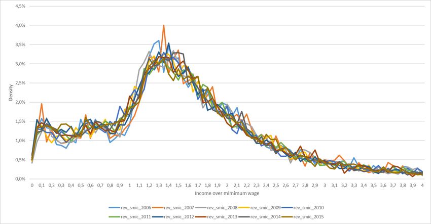
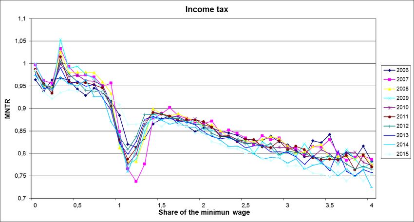
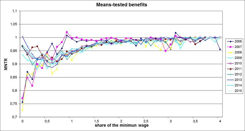
simulates each transfer by reconstructing the appropriate unit (home, tax-household, family,
household, and so on). It provides simulated transfers very close to the levels observed in the
administrative data.
After this first step, I can compute the marginal tax rates (MTR) of each tax and benefit, by
increasing labor income by 5% for each person and comparing the modified disposable income
with that in the counterfactual scenario. For households with more than one earner, the MTR
are calculated for each income earner by increasing each income by 5% in turn. Within the
same household, MTR may be different for each person in the household (husband, wife,
student children, etc.). This is an important difference with the ETI literature, which estimates
elasticities with respect to the MNTR at the tax household level.
Finally, since tax records also provide information on the labor income at t-1 and t-2, I can
compute the different instruments of the MNTR and ANTR by taking previous years' incomes
and applying the year's inflation to them.

 3.4. Descriptive statistics

Descriptive statistics of the basis for estimation are presented in Table A2 in Appendix B. It
shows that the marginal net of tax rates (MNTR) have a high standard deviation of 13 % of
labor income for income tax, 227 % for RSA and 7.1 % for family benefits. This strong
heterogeneity is also found in the annual variation of MNTR, whose standard deviation is
greater than 10% for each transfer. Table A2 also shows that the socio-demographic
characteristic of the sample reflects those of the working French population.38
Appendix B also displays the distributions of the ratio of labor income (z) to the annual
minimum wage for each year (Figure A2) and the distributions of simulated MNTR for income
tax and benefits for the different years (Figure A3). In these tables and figures, there is
variability from year to year at each point in the distribution, but it is difficult to determine
whether this heterogeneity reflects socio-demographic, income, or behavioral responses to tax
reforms. Several tax-related changes can be identified for MNTR. The lowest MNTR were in
2014, when there was a large reduction in income tax associated with a 100% MTR, and the
MNTR at the top of the distribution were lower after 2013, when the higher MTR were raised
(Figure A3.a). With regard to benefits (Figure A3.b), we clearly see the creation of the RSA in
2009, which reduced the MTR at the bottom of the distribution, and thus increased the MNTR
(and the opposite between 0.8 and 1.5 times the minimum wage in the phasing out of the RSA).

parliament at the end of income year t, it is impossible to adapt income of year t to future reforms of year t+1, and this static
policy expectation therefore seems credible. The second main change in the model concerns the take-up of the RSA benefit
schedule. Eligibility for RSA is simulated, but take-up is imputed using the social administrative data of the ERFS in this
study, and not randomly imputed as in the model INES. Indeed, in the INES model, the non take-up of certain benefits such
as the RSA is randomly imputed to achieve the administrative social data target.
38 38% had completed higher education, 75% worked in the tertiary sector, 84% worked full-time, 65% had a permanent

contract in a private company, 54% had been working in the same company for more than 10 years and 38% lived in a
municipality with a population of more than 200,000.

Reforms that have a different effect on households with the same income but different family
size39 do not show up in Figure A3, while they are an important source of identification. To get
a better idea of the source of our estimates, Table 1 shows the number of people facing a non-
zero predicted change in the MNTR of income tax and benefits (i.e., the change in the MNTR
instrument), decomposed by the magnitude of the change. This table shows, for example, that
37,557 people (about 40% of the sample) face a change in MNTR due (only) to income tax
reforms, and of these, 11,335 people (12% of the sample) face a change in their MNTR between
1% and 10%, 6,776 people face a change between 10% and 50% and 500 more than 50%.
Turning to means-tested benefits, 12,300 people face a change in the MNTR due to benefit
reforms (about 15% of the sample), nearly 2,000 face a decrease in their MNTR of more than
50%, and 1,200 face an increase of more than 50%. This heterogeneity of predicted variations
in MNTR can also be revealed by the high standard deviation of this variable in Table A2. The
many relatively large increases and decreases in the predicted variations of the MNTR are
important for econometric estimates because they imply that the tax variations used are not
systematically correlated with the level of income before the reform, which alleviate the issue
of mean reversion and heterogeneous income trend.
Table 1. Number of people facing a non-zero change in the MNTR income tax and benefit
instrument
 Changes in Income tax Means-tested benefits
 MNTR
 Inf. -50 % 633 1 952
 -50 % à -10 % 7 541 3 383
 -10 % à -1% 10 775 1 405
 1 % à 10 % 11 335 1 393
 10 % à 50 6 776 2 972
 Sup. 50 497 1 193
 Total 37 557 12 298
Reading note: 1952 people faced a decrease in benefit retention rates of more than 50% (equivalent to an increase of more than
50% in the marginal benefit rate)
Source: ERFS 2006-2015; INES model

 4. Results

In all estimates, the following transfers are taken into account: income tax (IT), RSA, and family
benefits (FB) including PAJE, ARS, FC and AF. 40 The reactions to MNTR are computed for
each of these transfers separately or grouped together (ALL). I first provide graphical evidence
(section 4.1), before turning to 2SLS estimation (section (4.2).

39
 For instance, reform of the family quotient in Figure 3, reform of the RSA in Figure 4, or reform of family allowances.
40They are grouped together because they do not have enough people separately. Other transfers (such as social security
contributions or housing allowances) are not taken into account because of the absence of any salient reform in the period.

4.1. Graphical evidence

I first provide graphical and semi-parametric evidence corresponding to first-stage and reduced-
form regressions. Since I use several different reforms as sources of variation, it enables me to
visualize the effect of MNTR on labor income. Indeed, unlike Kleven and Schulz who use
mainly one reform to identify the effect, I cannot use a graphical difference-in-difference to
highlight the effect.
Figures 5 and 6 plot a local fourth-order polynomial regression 41 of a variable Y on a variable
X. In each graph, the gray area represents a 95% confidence interval. These graphs are based
on Weber (2014) who first used them for the ETI estimation.42 Like Weber (2014), these graphs
depict polynomial regressions for predicted MNTR between -20% and +20%, which includes
more than 90% of the sample.43

Figure 5. Delta log of the MNTR according to the delta log of its instrument (first stage)

Notes: The figure represents a fourth-order local polynomial regression of the variation of the log MNTR on the variations of
the "predicted" log MNTR. No control variables included. The smoothing parameter is 0.09 (determined with AIC).
Source: ERFS 2006-2015

41
 I use the Epanechnikov kernel function for all polynomial regressions, associated with a polynomial order of four and a
bandwidth (calculated automatically by a Akaike Information Criterion (AIC)) of around 0.15 (depending on graphs).
42 Weber was not the first to use this non-parametric representation to investigate the effect of taxation: Bianchi et al. (2001)

provide graphical results of GAM (general-additive model) estimation for week work depending on tax rates to show the non-
linear effect of the pay-as-you earn reform in Iceland in 1987. Note that the graph of Weber is now commonly used in ETI
literature, for instance in Doerrenberg et al. (2017) and Hermle and Peichl (2018).
43 As Weber (2014) explains, "Extreme observations are excluded because the standard deviations on these observations are

large and make the rest of the graph difficult to read”.

A graphical illustration of the first step of the estimates in equation (9) is provided in Figure 5
for all transfers and for each separately. As expected, it shows a strong positive relationship
between the MNTR and its instrument, the predicted log change of MNTR (MNTR if incomes
were held constant). This positive relationship is almost linear for all transfers and income tax,
but less so for the RSA and family benefits (particularly at the top of the distribution of the
change of the instrument44).

Figure 6. Delta log of labor income as a function of the delta log of the predicted MNTR
(reduced form)

Notes: Graphical evidence of the reduced form of equation (9). The figure represents a fourth-order local polynomial regression
of the change in the logarithm of labor income to the changes in the logarithm of the MNTR predicted. No control variables
included. The smoothing parameter is 0.11 (determined with AIC).
Source: ERFS 2006-2015

Figure 6 provides a graphical representation of the reduced-form regressions. The relationship
between the change in the logarithm of labor income and the predicted log change of MNTR is
illustrated for all transfers, and for transfers in detail. The two variables are positively related
for all transfers, and for income tax and RSA. This reflects the positive elasticities that I estimate
econometrically in the next section and is consistent with a positive substitution effect. Since
the positive slope is steeper for income tax, the elasticity of income tax is expected to be higher
than that of benefits. For income tax, the relationship is strong for negative values and weaker

44
 This may be related to the fact that there are fewer individuals and the estimates are less robust at the extremities.