Does Reducing 'Underwaterness' Prevent Mortgage Default? Evidence from HAMP PRA
←
→
Page content transcription
If your browser does not render page correctly, please read the page content below
Does Reducing ‘Underwaterness’ Prevent Mortgage
        Default? Evidence from HAMP PRA∗
                 Therese C. Scharlemann† and Stephen H. Shore‡
                                          August 2013

                                             Abstract
          The Home Affordable Modification Program’s Principal Reduction Alternative
      (HAMP PRA) is a government-sponsored program to reduce the monthly mortgage
      payments and mortgage balances of struggling borrowers who are ‘underwater’, i.e.
      whose mortgage balance exceeds their home value. We use administrative data to
      examine the impact of principal forgiveness – a permanent mortgage balance re-
      duction – on subsequent mortgage delinquency. The program’s rules for allocating
      forgiveness imply two kinks (discontinuities in the first derivative) in the function
      that determines the amount of principal reduction as a function of the borrower’s
      initial negative equity level, ceteris paribus. On one side of each kink, increas-
      ing underwaterness leads on the margin to a dollar-for-dollar increase in principal
      reduction (holding the payment reduction constant by replacing other forms of pay-
      ment reduction with principal reduction); on the other side of the kink, increasing
      underwaterness does not change the mortgage modification on the margin. The
      impact of principal reduction can therefore be identified by exploiting the quasi-
      experimental variation in principal reduction using a regression kink design (RKD),
      comparing the relationship between underwaterness and default on either side of
      the kink. The quarterly hazard – the proportion of loans that become more than
      90 days delinquent and consequently exit the program – in our sample is 3.8%; we
      estimate that it would have been 4.7% in the absence of principal reduction, which
      averaged 29% of the initial mortgage balance.
          JEL Codes: G21 (Mortgages), R30 (Real Estate Markets, General)

    ∗
      We thank seminar participants at Georgia State University, Temple University, and the Office of
Financial Research.
    †
      U.S. Department of the Treasury; Office of Economic Policy. Views expressed in this paper do not
reflect those of the US Treasury.
    ‡
      Georgia State University; Department of Risk Management and Insurance.

                                                  1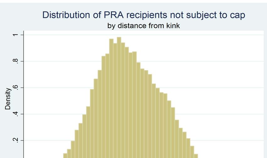
1        Introduction

There are more than 50 million first-lien residential mortgages in the U.S., with a total
balance exceeding $10 trillion. Mortgages represent by far the largest liability for U.S.
households.
    From the 4th quarter of 2006 through the first quarter of 2009, falling home prices
reduced U.S. home equity by nearly $5 trillion. As of the fourth quarter of 2012, an
estimated 10.4 million homes had negative equity or were ‘underwater’ (Corelogic, March
2013), with mortgage balances on those homes exceeding home values. Negative equity
on these underwater homes exceeded $800 billion at its peak, but had fallen to about
$628 billion by the fourth quarter of 2012. (Corelogic, March 2013) Research has raised
concerns that this negative equity may be associated with reduced mobility (Ferreira,
Gyourko, and Tracy, 2010, 2013)1 , an inability to refinance mortgages into the recent
low interest rate environment (Boyce, Hubbard, Mayer, and Witkin, 2012), and reduced
consumption (Mian and Sufi, 2011; Dynan, Spring 2012).
    During the same period that home prices fell and negative equity increased, mortgage
delinquency rates rose rapidly. The share of active mortgages in 90+ day delinquency or
foreclosure shot from 2.2 percent in the fourth quarter of 2006 to a peak of 9.7 percent
in the first quarter of 2010, though it has since fallen to 6.4 percent in the first quarter
of 2013. (Mortgage Bankers Association, May 2013) The possible link between negative
equity and mortgage delinquency is therefore of natural interest.
    This paper uses administrative data on the Home Affordable Modification Program’s
(HAMP’s) Principal Reduction Alternative (PRA) to examine the impact of principal
reduction on subsequent mortgage default, as measured by 90-day delinquency and con-
sequent disqualification from HAMP. For lenders and policy makers, this information is of
natural interest in designing mortgage modifications and in understanding the risks aris-
ing from various combinations of mortgage characteristics. (Das, 2012) For economists,
    1
        This result has been contested in Schulhofer-Wohl (2012).

                                                     2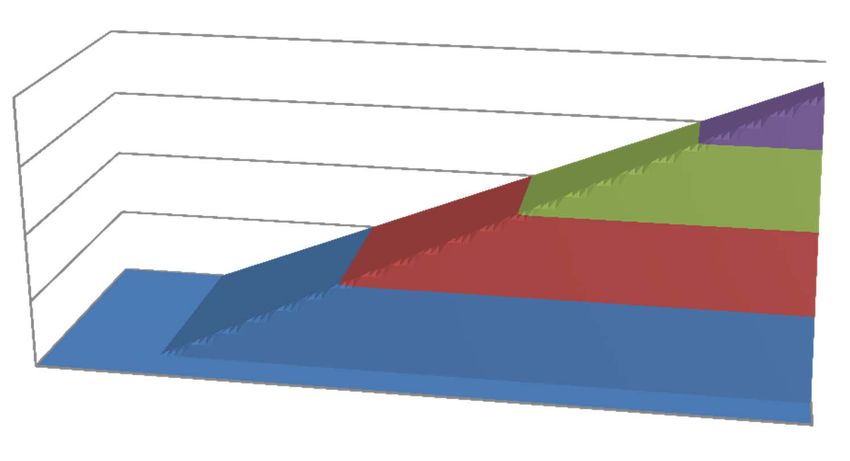
these findings contribute to the literature evaluating borrowers’ default decisions in the
context of negative equity (Foote, Gerardi, and Willen, 2008; Deng, Quigley, and van
Order, 2000).
    Several papers have examined the relationship between negative equity and mortgage
default since the start of the housing crisis (Bajari, Chu, and Park, 2010; Bhutta, Dokko,
and Shan, 2010; Fuster and Willen, 2012; Ghent and Kudlyak, 2011; Tracy and Wright,
2012; Haughwout, Okah, and Tracy, 2010). One strategy employed in the research is to
use loan-level performance data (Bajari, Chu, and Park, 2010; Bhutta, Dokko, and Shan,
2010) and exploit variation in negative equity arising from changes in state- or zip-code-
level home price indexes. Because certain information – such as income – is available
only at the time of origination, structural methods are used to control separately for
income shocks using available measures of local labor market conditions (e.g., state- or
county-level unemployment).
    The major challenge inherited by these research designs in the existing literature is
that the level of negative equity may not be exogenous. Variation in negative equity
driven by local price changes may be associated with having neighbors who are increas-
ingly underwater, living in an area with increasing vacancy rates, or low levels of home
maintenance. Variation in negative equity driven by initial downpayment, mortgage
terms, cash-out refinancing, or time of purchase may be associated with unobservable
borrower characteristics. Moreover, borrowers with different levels of negative equity
because they invested during different stages of the housing market may have been un-
observably different.2 As a result, using these sources of variation in negative equity may
not reveal the causal relationship between negative equity and mortgage default.
    Several papers have looked more directly at the role of principal reduction in mod-
ification performance by comparing the default rates on non-HAMP modifications with
   2
     For example, there is evidence that income was less-stringently documented as home prices acceler-
ated (Keys, Mukherjee, Seru, and Vig, 2010; Jiang, Nelson, and Vytlacil, 2011), and that second homes
comprised over half of the market near the height of the boom in areas with the most dramatic price
swings (Haughwout, Lee, Tracy, and van der Klaauw, September 2011).

                                                  3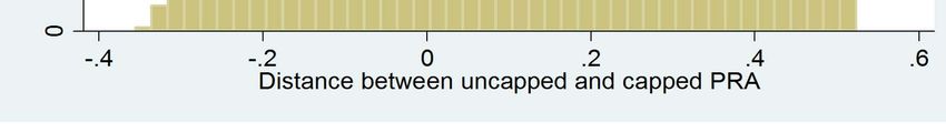
and without principal reduction. (Haughwout, Okah, and Tracy, 2010; Agarwal, Am-
romin, Ben-David, Chomsisengphet, and Evanoff, 2011) However, in these data, it is not
clear what unobservable criteria (including on variables like pre-modification DTI and
FICO that are observable in our data) affected who received principal reduction and how
much they received. Absent perfect controls, the impact of these unobservable factors on
mortgage default or delinquency may be misidentified as coming from negative equity.
   This paper aims to overcome the omitted variable bias problems that are unavoidable
when using local price variation to measure negative equity, as well as the selection issues
inherent in studies of non-random mortgage modifications. The structure of HAMP PRA
allows cleaner identification of the relationship between principal reduction and mortgage
default.
   The Home Affordable Modification Program (HAMP) Principal Reduction Alterna-
tive (PRA) is a government program to provide payment reduction and principal re-
duction to troubled mortgage borrowers whose mortgages are underwater. The HAMP
program is implemented by mortgage servicers, who can choose to participate. All poten-
tially eligible 60-day delinquent borrowers must receive a notice containing information
on applying for relief through HAMP. HAMP applicants provide information about their
income to calculate their mortgage debt-to-income ratio (DTI), a measure of the afford-
ability of a mortgage payment; an automated appraisal system is used to estimate the
borrower’s home value and with it their loan-to-value (LTV) ratio, a measure of negative
equity. The terms of a HAMP PRA modification are determined by the borrower’s initial
DTI, LTV, and a servicer-specific LTV target (usually 115% or 100%).
   HAMP PRA uses a series of specified mortgage modification steps to reduce mort-
gage payments until the borrower reaches a DTI ratio of 31%, the “affordability target”.
The first step uses principal forgiveness to reduce the mortgage balance to achieve the
affordability target, without reducing the borrower’s LTV below the servicer-specific tar-
get. Some servicers restrict the maximum principal reduction amount to 30% of the

                                             4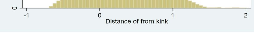
pre-modification unpaid balance. If principal reduction to the LTV-target is insufficient
to achieve the affordability target, the payment is decreased as needed until the afford-
ability target is reached by lowering the mortgage rate, extending the mortgage term,
and forbearing mortgage principal. Servicers evaluate modifications to determine their
net present value (NPV) to the lender before offering those modifications to borrowers.
   HAMP PRA program rules imply kinks – discontinuities in the first derivative – in the
function that determines the amount of principal reduction as a function of the borrower’s
initial negative equity, ceteris paribus. In a specific pre-modification LTV range, a higher
LTV generates a modification with more principal reduction (and less use of the other,
less generous modification steps). In this range, every additional dollar of unpaid balance
generates an additional dollar of principal reduction.3 However, for LTVs above this pre-
modification LTV range, a higher LTV has no effect on the mortgage modification terms.
We refer to the pre-modification LTV at the border between these ranges as the kink.
The pre-modification LTV at which this kink occurs varies from loan to loan based on
the affordability (DTI) of the initial mortgage and on the servicer-specific LTV target.
   Some loans are subject to a second kink because their servicer caps principal reduction
at 30% of the pre-modification principal balance. Below this 30% cap, increasing pre-
modification LTV and DTI increases principal reduction; above this cap, it does not.
   These kinks allow the impact of principal reduction to be identified by exploiting the
quasi-experimental variation in principal reduction from a regression discontinuity design
(RDD) (Hahn, Todd, and Van der Klaauw, 2001; Lee and Lemieux, 2010), or more
specifically a regression kink design (RKD) (Florens, Heckman, Meghir, and Vylacil,
2009; Card, Lee, Pei, and Weber, November 2012).4 We estimate the impact of principal
reduction on mortgage default by comparing the relationship between LTV and default
   3
      This is the pre-modification LTV range where reducing negative equity to its LTV target alone is
insufficent to reach the affordability target, namely DTI of 31%.
    4
      Provided the region around the kink is small enough and assignment on either side of the kink is
quasi-random, observable and unobservable variables should be the same for observations on either side
of the kink. As a result, additional controls are unnecessary and concerns about omitted variables are
lessened.

                                                  5
on either side of the kink.
Servicers are required to implement HAMP PRA based on explicit, observable, ob-
jective criteria, which we observe and can control for. This precludes, or at least limits,
servicer-based selection. Borrowers cannot observe their DTI or LTV with great preci-
sion, are unable to effectively manipulate LTV, and will typically not know their servicer’s
LTV target. Borrowers’ difficulty in determining on which side of the kink they will fall
at the time of HAMP application limits the scope for borrower-based selection into dif-
ferent principal reduction amounts. Finally, because we have loan-level information on
the borrower at the time of HAMP application, we can explicitly control for variables
(such as borrower DTI and FICO) that in other studies are unobservable or observable
only at origination.
We find that principal reduction reduces subsequent rates of delinquency. Among
HAMP PRA participants in our sample, 3.8% become at least 90 days delinquent (at
which point they are dropped from the program) per quarter on average. Our estimates
suggest that this rate would have been 4.7% (95% confidence interval (CI): 4.3% to
5.2%) had these borrowers received modifications with no principal reduction (but the
same payment reduction, achieved instead through rate reduction, term extension, and
principal forbearance). The average loan in the HAMP PRA sample received a 29%
reduction in the mortgage balance. The first cohort of PRA modifications in our sample
(originated 2011:Q1) had a cumulative default rate of 31%; we estimate that their default
rate would have been 40% (95% CI: 36% to 44%). The cumulative default rate in the
sample (overall default rate thus far) is 15.8%; we estimate that it would have been 19.2%
(95% CI: 17.8% to 20.9%).
These results are robust to a variety of specifications and are present in various
sub-samples of the data. Furthermore, separate analyses of the two kinks yield similar
estimates of the impact of principal reduction on subsequent default. We find some
evidence that the impact of principal reduction on default abates somewhat for later
6cohorts.
2 HAMP Structure and Identification
The Home Affordable Modification Program (HAMP) was announced in February 2009,
under the authority of the Troubled Asset Relief Program (TARP). HAMP subsidizes
servicers and lenders to modify mortgages according to the terms of a HAMP modifi-
cation. At the beginning of the program, participating services were required to sign a
Servicer Participation Agreement (SPA), which obligates them to comply with HAMP
protocols on all of the loans in their servicing portfolio, to the extent permitted by their
pre-existing contracts with mortgage investors. Servicers covering nearly 90% of the
mortgage market elected to participate in the HAMP program, though not all of these
services elected to participate in the Principal Reduction Alternative (PRA).
HAMP requires services to send borrowers a letter with information on applying for
a HAMP mortgage modification when they become 60-days delinquent.5 To be eligible
for the HAMP program, borrowers must have a mortgage DTI over 31%, live in the
mortgaged home, and have an unpaid balance below $729, 750; however, larger balances
are allowed for multi-family properties if the borrower lives in one of the units.6 Bor-
rowers must sign a hardship affidavit, under penalty of perjury, stating that they have
experienced a hardship and are unable to make their current mortgage payments.
When borrowers apply for HAMP, they provide information about their income, which
is used to determine the debt-to-income (DTI) ratio, the measure of affordability used by
HAMP. DTI measures the fraction of the borrower’s pre-tax income that goes to monthly
5
Non-delinquent borrowers may also apply for HAMP, and are eligible for the program if their default
is deemed imminent. Though many servicers use an imminent default calculator similar in structure to
the default model embedded in the HAMP NPV test, ultimately imminent default is determined by the
servicer for their and their investors’ portfolios.
6
In June 2012, HAMP eligibility was expanded to non-owner occupiers, borrowers with lower DTI
ratios, and borrowers who could not achieve a 31% DTI ratio using the standard HAMP modification
steps. The modification granted by the expanded program (HAMP Tier 2) is different than in the
original program and does not generate the kink employed in our identification strategy, even when
principal reduction is included. We exclude PR recipients in Tier 2 from our sample.
7first-lien mortgage payments, real estate taxes, homeowner’s insurance, and condominium
or homeowner’s association dues. Temporary income – such as from unemployment
insurance – is excluded from the gross income calculation. An automatic appraisal system
calculates home value, which is used to determine the loan-to-value (LTV) ratio – the
balance on the first mortgage divided by the home value – which is the measure of home
equity used by HAMP. Updated FICO scores are pulled from credit bureaus.
Two modifications are commonly offered under HAMP: ‘Standard’ HAMP and HAMP
PRA. Servicers use an NPV model to compare the expected discounted cash flows lenders
would receive under each potential modification and without a modification. The NPV
model estimates a default probability, prepayment rate, and recovery rate based on the
borrowers’ pre- and post-modification DTI and LTV, their FICO score and delinquency
at the time of modification, their geography, and other variables. Servicers typically offer
borrowers the option that yields the highest NPV, though they may use other objective
criteria (e.g., do a HAMP PRA modification if it is better than no modification even if
‘Standard’ HAMP yields an even higher NPV).7 Not all HAMP-participating servicers
participate in HAMP PRA, and some loans serviced by HAMP PRA-participating ser-
vicers are ineligible for HAMP PRA (e.g., loans guaranteed by Fannie Mae and Freddie
Mac, and mortgage investors whose contracts specifically forbid or limit principal for-
giveness).
Once borrowers are offered and accept the modification, they are given a three-month
trial period during which they must stay current on their new, lower mortgage payments
and produce any required documentation (e.g., occasionally certain income documents are
not collected up front). If borrowers fail to produce this documentation or go delinquent
during this period, they fail out of the trial modification. At this point, the mortgage
7
While there will be selection into ‘standard’ HAMP, HAMP PRA, and no modification based on
the NPV model, the structure of the model is known to the econometricians (and is publicly available at
www.hmpadmin.com) as are the loan-level variables used to calculate the NPV for each borrower who
receives a HAMP PRA modification. As a result, any selection stemming from the NPV model can be
corrected for explicitly.
8reverts to its pre-modification terms and delinquency or foreclosure proceedings can con-
tinue; the borrower may also be evaluated for a non-HAMP modification. The mortgage
modification becomes permanent after the trial period, at which point delinquency or
foreclosure proceedings are terminated. If borrowers become more than 90 days delin-
quent on a permanent modification, they are dropped from the program and delinquency
or foreclosure proceedings can be re-initiated; mortgage terms will nominally remain as
specified in HAMP unless the servicer elects to further modify the borrower.
To encourage participation in HAMP, the government provides subsidies to participat-
ing lenders, servicers, and borrowers. Servicers receive an up-front fee for each permanent
modification ($400-$1,600) plus up to $1,000 per year for each year that a modification
remains in the program (up to 5 years). Borrowers receive up to $1,000 per year if the
borrower remains in the program (up to 5 years), applied directly to their unpaid bal-
ance, as long as they are not delinquent. Lenders receive half of the borrower payment
reduction between 38% and 31% DTI while the borrower is in the program (up to 5
years). These payments apply to all HAMP modifications, both ‘standard’ HAMP and
HAMP PRA. Investors also receive subsidies for writing down principal, which we cover
in the section below.
2.1 ‘Standard’ HAMP
The standard HAMP modification is designed to bring the borrower’s mortgage payment
to an affordable level, defined in this program as a post-modification DTI of 31%. Bor-
rowers with a pre-modification DTI below 31% are ineligible for HAMP; borrowers with
a pre-modification DTI above 31% have their post-modification DTI reduced to 31%.
Past-due fees are waived and past-due interest is capitalized into the unpaid mortgage
balance. The standard modification does not permanently reduce the mortgage balance
and is not the focus of this paper.
The standard HAMP modification is summarized in Table 1. The payment reduction
9in the standard modification is achieved first by reducing the mortgage interest rate until
the payment hits the affordability target of 31% DTI or the rate hits the 2% floor. If
further payment reduction is needed to reach 31% DTI, the mortgage term is extended in
monthly increments until the payment reaches 31% DTI or the term reaches 40 years. If
further payment reduction is needed to reach 31% DTI, then principal forbearance is used
as needed to reach 31% DTI (which is equivalent to reducing the interest rate as needed to
zero). Servicers may cap principal forbearance at 30% of the borrower’s principal balance;
if the payment target cannot be met using 30% principal forbearance, the borrower can
be turned down. The mortgage terms remain unchanged for five years; after five years,
if the modified mortgage rate is below the Primary Mortgage Market Survey (PMMS)
30-year fixed-rate-mortgage rate that prevailed at the time of the modification (the rate
cap), the mortgage rate rises one percentage-point per year until it reaches the rate cap,
at which point it becomes fixed. Borrowers with modification rates over the rate cap
retain their modification rate for the duration of the modified mortgage term.
2.2 HAMP PRA
The HAMP Principal Reducation Alternative (PRA) modification is designed to bring
the borrower’s mortgage payment to an affordable level – to a post-modification DTI of
31%, like ‘standard’ HAMP – in a way that prioritizes principal reduction, as summa-
rized in Table 1. Standard HAMP and HAMP PRA therefore involve the same payment
reduction, though PRA modifications achieve at least some of that payment reduction by
reducing the principal balance. Servicers set their own LTV targets for HAMP PRA. Ser-
vicers covering roughly three-quarters of our sample use a 115% target, and the remaining
use 100%.8
8
Some borrowers are ineligible for PRA, including borrowers with an LTV below the target, borrowers
with loans guaranteed by Fannie Mae or Freddie Mac, and loans in securitization pools that explicitly
prohibit principal reduction. While many servicers did not participate in PRA initially, most non-GSE
HAMP modifications are done by servicers who now participate in PRA. We have excluded several
PRA-participating services with volume so low we could not ascertain their LTV target with certainty,
and one large servicer who uses a principal-reduction allocation method that does not generate the kink
10Payment reduction is achieved by reducing mortgage principal until the borrower’s
payment achieves the affordability target (31% DTI) or the borrower’s LTV reaches the
servicer’s target, whichever requires less principal reduction.9 Servicers with an LTV
target of 100% have also chosen to apply a 30% cap on the amount of principal reduction
as a share of the principal balance. If the affordability target of 31% DTI is reached
using principal reduction, the borrower’s LTV remains at or above the servicer’s LTV
target, and there are no further steps in the modification; in this range, increasing pre-
modification LTV on the margin would have no effect on the mortgage modification. If the
affordability target of 31% DTI has still not been reached when LTV has been reduced
to its target level, then the modification proceeds using the steps from a ‘standard’
HAMP modification. The interest rate is reduced as needed to reach 31% DTI or to
2%, whichever comes first; then if needed, the mortgage term is lengthened as needed to
reach 31% DTI or 40 years, whichever comes first; then, principal is forborne as needed
to reach 31% DTI. In the range where principal reduction alone is insufficient to achieve
the servicer’s LTV target, increasing pre-modification LTV on the margin would lead
to more principal reduction (a larger percent change in LTV) and correspondingly less
temporary rate reduction, term extension, or forbearance, whichever is the last step in
the modification reached by that borrower.
Nominally, the principal reduction is phased in over three years in three equal-sized
increments. However, if the borrower wishes to sell or refinance the house at any time,
they need repay only the post-modification loan balance, which incorporates the full
forgiveness amount. If the borrower becomes more than 90 days delinquent and is kicked
out of the HAMP program, their balance is reduced by only the portion of the principal
we exploit for identification.
9
One major servicer implements HAMP PRA using a different formula. HAMP provides flexibility
for servicers to lower payments below 31% DTI. This servicer reduces the mortgage principal until the
borrower’s LTV reaches the servicer’s target, regardless the DTI reduction. If the LTV target is achieved
at a DTI above the affordability target required by HAMP, the standard HAMP waterfall is employed
to achieve the remainder of the payment reduction. This servicer is excluded from this analysis because
the kinks we study here are not present in their principal reduction formula.
11reduction that they ‘earned’ from their time in the program, not the full amount. Any
remaining PR that has not been vested is converted to forbearance.
To provide lenders with an incentive to participate in HAMP PRA, principal forgive-
ness is subsidized. Originally, the subsidy was $0.21 per dollar of principal reduction in
the LTV range above 140%, $0.15 per dollar of principal reduction in the LTV range
between 115 % and 140%, and $0.06 per dollar of principal reduction in the LTV range
between 105% and 115%. These lender subsidies for principal reduction were tripled
by the government in March 2012 to encourage lender participation in the program, so
that current subsidies now range from $0.18 to $0.63 per dollar of principal reduction.
Borrowers who are more than 6 months delinquent at the time of modification receive
the lowest level of subsidy, regardless the LTV of the principal forgiven. Subsidies are
granted over three years as principal is nominally forgiven/earned (not up-front), or upon
borrower prepayment; as a result, lenders receive no subsidy on borrowers who default
immediately.
Table 1: ‘Standard’ HAMP and HAMP PRA Modifications
Standard HAMP
HAMP PRA
No reduction Reduce mortgage balance as needed
in mortgage balance to reach the lesser of
underwaterness target
(typically 115% LTV) and
affordability target (31% DTI)
If previous step insufficient to reach 31% DTI, then
reduce interest rate down to 2% as needed to reach 31% DTI.
If previous step insufficient to reach 31% DTI, then
extend loan term to up to 40 years as needed to reach 31% DTI.
If previous step insufficient to reach 31% DTI, then
foerbear principal as needed to reach 31% DTI.
(equivalent to zero rate)
122.3 Identification
The structure of the HAMP PRA modification includes two kinks that we exploit for
identification. On one side of each kink, the principal reduction amount varies with
the borrower’s LTV, while on the other side, the modification structure is invariant to
LTV. While HAMP PRA loans differ in their pre-modification affordability (as measured
by DTI), all HAMP PRA modifications have the same post-modificiation affordability
level.10 Post-modification LTV (or equivalently, the amount of principal reduction (PR))
will depend on pre-modification LTV, the servicer’s LTV target, the pre-modification
mortgage DTI (pre-modification MDTI), and the mortgage DTI target (MDTI target)
as follows:11
pre-modification LTV
PR ≡ −1 (1)
post-modification LTV
pre-modification LTV pre-modification MDTI
= max 0, min , −1 .
target LTV target MDTI
Limiting the sample to loans with a pre-modification LTV above their servicer’s target
and taking logs yields:
ln (1 + PR) = min(ln pre-modification LTV − ln target LTV, (2)
ln pre-modification MDTI − ln target MDTI).
The amount of principal reduction (PR) is a kinked function of the borrower’s pre-
10
The total DTI target is 31% on all loans. Borrowers may differ in their ability to pay 31% of
income for housing based on other credit card debts, student loan payments, health expenditures, or
other obligations.
11
The servicer LTV target is 115% for 75% of loans and 100% for the remaining 25%. DTI is the
proportion of income needed for the mortgage payment and other fixed housing expenses such as real
estate taxes, homeowner association fees and insurance. DTI is the sum of the mortgage DTI (MDTI)
and the fixed DTI (FDTI), where the former is the proportion of income needed to make the mortgage
payment and the latter is the proportion of income needed to pay real estate taxes, insurance, and other
fixed housing expenses, which do not vary with the mortgage terms. Since the mortgage modification
does not change the fixed portion of the borrower’s monthly payments, the 31% DTI target must be
achieved exclusively by reducing the mortgage DTI. As a result, the mortgage DTI target is 31% minus
the pre-modification fixed DTI.
13modification LTV. The location of the kink depends on the pre-modification MDTI, the
servicer’s target LTV and the borrower’s target MDTI. The pre-modification LTV at the
kink equates the two arguments of the min function in equation (1):
pre-modification MDTI
pre-modification LTV? = target LTV × (3)
target MDTI
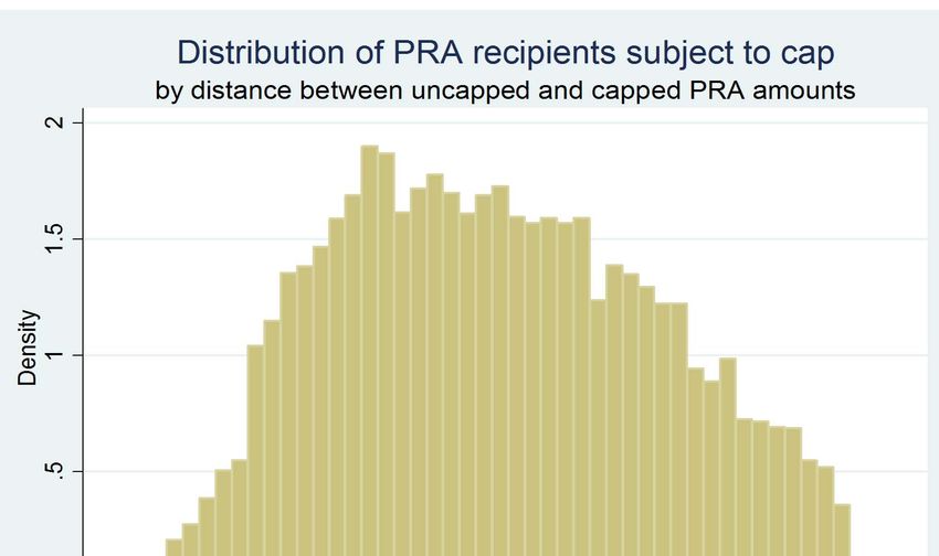
For pre-modification LTVs below LTV*, the amount of principal reduction included
in the modification is increasing in pre-modification LTV (and the amount of tempo-
rary rate reduction or term extension is decreasing in pre-modification LTV); for pre-
modification LTVs above LTV*, the mortgage modification terms do not depend on the
pre-modification LTV:
d ln(1 + PR)
=1 if pre-modification LTV < pre-modification LTV?
d(ln(pre-modification LTV))
=0 (4)?
if pre-modification LTV > pre-modification LTV
A second kink is present at the 30% principal reduction (PR) cap for roughly one-
quarter of mortgages with servicers that apply this cap.12 The cap lowers pre-modification
LTV* in equation (5) for high-DTI, high-LTV borrowers. Below the pre-modification
LTV* implied by this cap, increasing LTV increases principal reduction; above this point,
the modification is unchanged by increasing LTV.
12
For loans with servicers who have a LTV target of 100%, principal reduction is limited to 30% of
the initial mortgage balance. In this case, PR ≡ 1/(1 − 30%) − 1 = 10/7 − 1 = 3/7 . For this sample,
the principal reduction amount is determined as follows:
pre-modification LTV
PR ≡ −1 (5)
post-modification LTV
pre-modification LTV pre-modification MDTI
= max 0, min , , 10/7 − 1 .
target LTV target MDTI
Limiting the sample to loans with LTV above their servicer’s target and taking logs yields:
ln (1 + PR) = min(ln 10 − ln 7, ln pre-modification LTV − ln target LTV, (6)
ln pre-modification MDTI − ln target MDTI).
14The kinked structure of the problem allows us to examine the impact of principal re-
duction while controlling separately (and even non-parametrically) for pre-modification LTV,
pre-modification MDTI, and target LTV, and target MDTI. This suggests the following
basic regression to predict re-default:
Pr(Default) = f (α + βPR ln (1 + PR) (7)
+ βLTV (ln pre-modification LTV − ln LTV target)
+ βDTI (ln pre-modification MDTI − ln MDTI target)
+ βX X + ε)
The principal reduction term in the first row of equation (7) is the minimum of the terms
found in the second (the negative equity term) and third rows (the affordability term).
The regression examines the impact of principal reduction while controlling separately for
the variables that determine it. The identifying assumption here is that this minimum of
the affordability term and the negative equity term has no independent impact on default
except insofar as at determines the amount of principal reduction the borrower receives.
It is straightforward to allow for an interaction of the negative equity and affordability
terms, so long as this interaction doesn’t take the kinked form of a minimum.
As is standard in a regression kink framework, βLT V and βDT I control for the bor-
rower’s position relative to the kink, and βP R gives the change in the slope at the kink
point. The change in the reaction function at the kink point must be divided by the
change in the derivative of the treatment function at the kink point, which in this case
is one.
We control for the number of quarters that have passed and the servicer’s LTV target
in every specification. Additional controls including servicer dummies, calendar quar-
ter dummies, LTV target dummies, ln(pre-modification DTI), geographic information,
income, balance, fico, and NPV test outcomes can be added, and a variety of para-
15metric specifications can be included. Furthermore, we can perform the analysis in the
neighborhood around the kink, where:
pre-modification LTV
abs lnFigure 1: HAMP PRA Identification
Without Principal Reduction Cap
Moderate Payment Reduction Needed Large Payment Reduction Needed
to Reach DTI Target to Reach DTI Target
Final LTV (red)
Final LTV (red)
unt unt
o o
Am Am
PR PR
DTI limits PR
DTI limits PR
LTV Target
LTV Target
45º 45º
Initial LTV Initial LTV
With Principal Reduction Cap
Moderate Payment Reduction Needed Large Payment Reduction Needed
to Reach DTI Target to Reach DTI Target
Final LTV (red)
Final LTV (red)
nt
unt ou
o m
Am A
PR PR
Have Limited PR
Cap limits PR
DTI limits PR
LTV Target
DTI Would
LTV Target
45º 45º
Initial LTV Initial LTV
See text for details.
17to target).
Figure 2: Principal Reduction Amount
0.8
0.6
0.4
0.2
49
0
37
100
106
112
118
124
130
136
142
148
25
154
160
166
172
178
184
190
196
underwaterness (loan‐to‐value)
3 Data
Data come primarily from HAMP administrative “loan setup” files, which record mod-
ification characteristics and performance. Additional data come from “NPV run” files,
which record variables used when evaluating the net present value of modifications to
the lender.13 We examine new permanent HAMP modifications on non-GSE loans (GSE
loans are those guaranteed by Fannie Mae or Freddie Mac, which are ineligible for HAMP
PRA) enrolled in 2011 and 2012.
HAMP PRA officially launched in October 2010, but borrowers must complete a 3-
month trial period before becoming eligible for an “official” modification, which entitles
the borrower, servicer, and investor to government subsidies, and which permanently
alters the borrower’s mortgage terms. We therefore begin our sample in January 2011.
We focus on modifications that complete the trial period and become permanent because
13
Not all records in the loan setup files have matching NPV run files; when we include variables from
the loan set-up file in our regressions, some observations are dropped.
18these data are checked for internal consistency and randomly audited as the subsidy
payments are set up. Data on loans that fail out of the trial period are not subject
to this level of scrutiny, and are often unreliable. About 10% of the trial modifications
originated during our sample period failed to become permanent; roughly two-thirds of
this fall-out can be attributed to nonpayment. Because we cannot consistently decipher
whether the failure to submit documentation reflects ineligibility or default, we do not
consider the impact of principal reduction on re-default in the first three months of a
modification; results are conditional on the modification’s survival to three months.
We use falling 90 days (or more) delinquent – and consequent disqualification from
HAMP – as our measure of default.14 This is similar to the default measure used by
Bhutta, Dokko, and Shan (2010). We have no subsequent performance data on borrowers
who drop out of HAMP. Our analysis is performed at a quarterly frequency, examining
the default hazard in each calendar quarter for cohorts of loans that became permanent
in each calendar quarter.15 Because it takes 90 days to be dropped from HAMP due to
delinquency, it is virtually impossible to exit HAMP in the same quarter that a permanent
modification begins. As a result, we include default data from the second quarter of 2011
through the first quarter of 2013. The first cohort of modifications (those that became
permanent in the first quarter of 2011) have eight quarters of default data (from the
second quarter of 2011 through the first quarter of 2013); the most recent cohort of
modifications (those that became permanent in the fourth quarter of 2012) have only
one quarter of default data (the first quarter of 2013).
14
After being kicked out of HAMP, the borrower may be evaluated for an additional non-HAMP
modification, or foreclosure proceedings may be initiated. We do not have loan-level performance data
following disqualification, so the eventual disposition of disqualified PRA HAMP modifications is unob-
served. We refer to falling out of the program as “default” or “re-default”, but borrowers falling out of
HAMP do not necessarily permanently default – their mortgage could be repaid in full outside of HAMP.
However, it is worth noting that falling out of HAMP PRA is punitive – the borrower loses any principal
forgiveness that has not yet been earned. Because of the earned principal reduction feature, HAMP
PRA is more generous than nearly all modifications available to borrowers, so a borrower who fails out
of HAMP PRA is unlikely to remain in their home as a homeowner without a material improvement in
their financial position.
15
Default is recorded in the quarter in which the loan first becomes 90 days delinquent, namely 90
days after the last payment the borrower was scheduled to make but did not.
19Table 2: Summary Statistics About Loans and Borrowers
N Median Mean St. Dev. Min Max
Balance pre-mod (0 000s) 46,343 $289 $322 $173 $10 $1,279
Home value (0 000s) 46,343 $175 $202 $116 $7 $856
Gross monthly income (0 000s) 46,343 $4.4 $4.9 $2.4 $0.6 $22.2
Total Mortgage Payment (0 000s) 46,343 $2.0 $2.2 $1.1 $0.3 $9.5
Principal & Interest Payment (0 000s) 46,343 $1.6 $1.8 $0.9 $0.2 $9.0
FICO 43,423 556 563 68 250 839
The mortgage balance includes accrued past unpaid interest; the home value is the assessed home
value from the servicer’s automated valuation model (AVM) at time of modification, or a broker’s
price opinion (BPO) or appraisal, where an AVM is unavailable. Monthly mortgage payment includes
mortgage principal and interest; monthly total payment includes mortgage principal and interest, as
well as homeowners’ insurance premiums and property taxes. Gross income is the borrower’s monthly
pre-tax eligible income, excluding temporary sources such as unemployment insurance benefits or self-
employment income from an irregular source. The sample includes most borrowers who received some
amount of principal reduction through the HAMP PRA program between January 1, 2011 and December
31, 2012. The sample excludes borrowers who received unsubsidized principal reduction (which may be
allocated under a different framework than PRA) and borrowers whose servicers’ PRA policies either
could not be imputed or did not generate the kink exploited for this analysis.
We encounter extreme values in the data, some of which likely reflect data entry errors
rather than true mortgage characteristics. On these grounds, we exclude borrowers with
initial total DTI over 100% and initial LTV over 240%. We drop loans for which either
the mortgage rate, term, or unpaid balance is recorded as zero, or where servicers PRA
policies could not be determined because they had very few PRA loans. We also drop
loans that received principal reduction through a program other than HAMP PRA. We
drop one large servicer who uses a principal-reduction allocation method that does not
generate the kink we exploit for identification; loans from this servicer are a majority of
dropped loans. The dropped population comprised about 50% of the full sample of PRA
recipients who enrolled during the sample period. For these reasons, our total loan counts
will not match publicly-available information on the HAMP PRA program. During the
enrollment period in our sample, 532,052 new permanent modifications were started in
HAMP. Of these, 89,217 included HAMP PRA principal forgiveness amounting to $7.1
billion. Our sample consists of 46,343 loans, and $3.7 billion in principal forgiveness.
20Figure 3: Loan Count Statistics
Cumulative Default Rate over Time, by Quarter of Modification Cumulative Default Rate by Quarter of Modification
10,000 35%
35% Quarter of
modification 9,000
30%
30% 8,000
2011:Q1
7,000 25%
25% 2011:Q2
6,000
2011:Q3 20%
20%
5,000
2011:Q4 15%
15% 4,000
2012:Q1 3,000 10%
10%
2012:Q2 2,000
5%
5% 1,000
2012:Q3
0 0%
0% 2012:Q4
2011:Q1 2011:Q2 2011:Q3 2011:Q4 2012:Q1 2012:Q2 2012:Q3 2012:Q4 2013:Q1 2011:Q1 2011:Q2 2011:Q3 2011:Q4 2012:Q1 2012:Q2 2012:Q3 2012:Q4
Quarter of Modification Quarter of Modification
Count of loans modified in quarter x (red bars, left axis)
Proportion of modifications that have exited through 2013:Q1 (green line, right axis)
Hazard by Calendar Quarter Hazard by Quarters Since Modification
(Quarterly rate of exit from program) (Quarterly rate of exit from program)
45,000 5.0% 50,000 5.0%
40,000 4.5% 45,000 4.5%
35,000 4.0% 40,000 4.0%
3.5% 35,000 3.5%
30,000
3.0% 30,000 3.0%
25,000
2.5% 25,000 2.5%
20,000
2.0% 20,000 2.0%
15,000
1.5% 15,000 1.5%
10,000 1.0% 10,000 1.0%
5,000 0.5% 5,000 0.5%
0 0.0% 0 0.0%
2011:Q1 2011:Q2 2011:Q3 2011:Q4 2012:Q1 2012:Q2 2012:Q3 2012:Q4 1 2 3 4 5 6 7 8
Quarters since Modification
Count of loans in calendar quarter (red bars, left axis) Count of loans in sample x quarters after modification (red bars, left axis)
Hazard in calendar quarter (green line, right axis) Hazard in quarter that is x quarters after modification (green line, right axis)
Figure 3 and 4 present information about counts, rates of HAMP exit following 90
days of delinquency, and sample attributes. Table 2 describes the borrowers and their
loans before modification. Table 3 describes summary statistics about the modification
terms.
Table 2 shows that the median home value in the sample is $175, 000 and the median
pre-modification mortgage balance is $289, 000, though there is substantial variation.
Table 3 shows that HAMP PRA reduces the median DTI from 44% to 31% and reduces
median LTV from 160% to 115%, a 30% reduction in principal on average. Figures 3
(upper right corner) shows that the number of new modifications peaked in the third
quarter of 2011 at just under 10, 000 for the quarter and has fallen consistently since
then to below 4, 000 in the most recent quarter.
Figure 4 shows that roughly three-quarters of loans in the sample have servicers
21Figure 4: Summary Statistics
LTV target Rate Type
115% LTV Target,
Fixed Rate
no PR cap
100% LTV target,
Adjustable Rate
30% PR cap
Lender Type Limiting Factor for Modification
Securities DTI Target Binds
Investor LTV Target Binds
Bank Portfolio PR Cap Binds
with a 115% LTV target; none of these servicers have elected to place a cap on the total
allowable amount of principal reduction; servicers for the remaining quarter of loans have
a 100% LTV target; all of these servicers have elected to place a 30% cap on the principal
reduction amount. Slightly more loans in the data have fixed rates than adjustable rates,
and the majority of loans are held in mortgage backed securities and not held on bank
balance sheets. In roughly two thirds of all cases, the LTV target is the limiting factor
determining the amount of principal reduction received; reducing the mortgage balance
until the LTV target is met is insufficient to reach the affordability target, and rate
reduction (as well as possibly term extension and forbearance) are needed to reach the
affordability target.
Figures 3 shows that default rates have been relatively constant as modifications age,
22Table 3: Summary Statistics About Modification
N Median Mean St. Dev. Min Max
Total DTI pre-mod 46,343 44.3% 47.1% 12.3% 29.4% 100.0%
Total DTI post-mod 46,343 31.0% 31.0% 0.3% 19.8% 32.9%
Total payment reduction 46,343 29.9% 30.0% 16.1% 0.0% 69.0%
LTV before modification 46,343 159.8% 164.8% 33.6% 109.8% 240.0%
LTV after modification 46,343 115.0% 121.6% 16.8% 100.0% 237.7%
Principal balance reduction 46,343 29.7% 29.1% 16.7% 0.0% 73.5%
Rate pre-mod 46,343 6.5% 6.4% 2.0% 0.0% 15.1%
Rate post-mod 46,343 3.0% 3.9% 2.2% 1.0% 15.0%
Term pre-mod (months) 46,343 305 317 59 1 541
Term post-mod (months) 46,343 302 330 73 12 541
Mortgage debt-to-income (DTI) is the ratio of the mortgage payment (principal and interest) to gross
income. Total DTI is the ratio of the total payment ( principal, interest, homeowners insurance, and
property taxes) to gross income. Loan-to-value (LTV) is the ratio of the mortgage balance to the home
value.
with a hazard of about 4% per quarter between the second and eighth quarters after
modification. There is some indication that default rates have fallen with calendar time
– from a peak in the quarterly default hazard in the fourth quarter of 2011 at 4.7% to
3.6% in the first quarter of 2013 – though the relationship is not monotonic.
Because the identification strategy relies on a kink in the principal reduction formula,
it is critical that the amount of principal reduction received actually adhere to that
formula. PRA participants receive almost exactly the amount of principal reduction
predicted by the program. A regression to predict the natural log of actual principal
reduction with the natural log of predicted principal reduction and no other covariates
has a precisely-estimated coefficient of 1.007 and an R2 of 0.98. While the analyses that
follow examine the relationship between predicted principal reduction (given the program
design outlined in Section 2) and default, results are nearly identical when actual principal
reduction is used instead.
23Table 4: Quarterly Hazard: Impact of Principal Reduction on Program Exit
Dep. Var. Program exit, becoming 90+ days delinquent (quarterly)
ln(predicted PR) -0.350*** -0.247*** -0.284*** -0.271*** -0.306***
(0.057) (0.058) (0.059) (0.068) (0.107)
ln(PR from LTV) 0.202*** 0.145*** 0.005 0.227*** -0.052
(0.039) (0.040) (0.053) (0.061) (0.309)
ln(PR from DTI) -0.429*** 0.249*** 0.141*** 0.162*** 0.630*
(0.019) (0.023) (0.036) (0.049) (0.339)
Controls
LTV target = 115 percent? YES YES YES YES YES
Quarters since mod YES YES YES YES YES
Quarter of mod NO YES YES YES YES
Total DTI pre-mod NO YES YES YES YES
Interaction variable NO NO YES YES YES
Other controls NO NO NO YES YES
10-ppt LTV and DTI bins NO NO NO NO YES
Observation Count 193,001 193,001 193,001 167,428 167,090
Loan Count 46,343 46,343 46,343 40,765 40,661
R2 0.025 0.046 0.047 0.079 0.080
Each observation refers to a loan in a calendar quarter; observations are included on loans that have
not exited from the program to date and for which data is available for the entire quarter. Since
program exit is nearly impossible in the quarter in which a loan was modified, observations begin
in the quarter following the quarter of modification. The regression shows results from a hazard for
quarterly program exit, where the hazard is specified as a probit; coefficients are shown. “Quarter
since modification controls” indicate dummy variables for the number of quarters since the modification;
“quarter of modification controls” are dummy variables for the calendar quarter in which the loan was
modified. Total DTI controls for the natural log of the pre-modification total debt-to-income (DTI)
ratio. The interaction control is a control for the interaction of the natural logs of pre-modification total
DTI and pre-modification loan-to-value (LTV). “Other Controls” includes FICO score, adjustable rate
mortgage dummy, investor-owned mortgage dummy, ln income, ln pre-modification mortgage balance,
length of trial modification (linear and squared), ln NPV of HAMP modification over no modification, ln
NPV of HAMP PRA modification over no modification, and a dummy for whether the standard HAMP
modification had a higher NPV than the HAMP PRA modification.
244 Results
Table 4 shows the results of the probit regression in equation (7) to predict the quarterly
default hazard using the natural log of the amount of principal reduction (PR, predicted
by equations 1 and 5) and additional controls. The first column includes linear controls
for the natural log of the principal reduction amount predicted by the borrower’s LTV
and the natural log of the PR amount predicted by DTI (which combined control for the
location of the kink), an indicator variable for whether the servicer uses an LTV target
of $115 (as opposed to 100%), and 8 dummy variables indicating the number of quarters
since modification. The second column adds 8 dummy variables indicating the modifica-
tion’s cohort quarter, the borrower’s and the borrower’s pre-modification total DTI. The
third column adds an interaction between the natural log of LTV and the natural log of
DTI. The fourth column adds additional controls, including servicer dummies, state dum-
mies, the borrower’s FICO, NPV test results (for standard and PRA, in natural logs),
the natural log of gross monthly income, the natural log of pre-modification principal
balance, the trial length (in months), the square of the trial length, and dummy variables
indicating ARM and investor-owned loans. The final column adds 10-percentage-point
bins for each of the PRA reduction predicted by LTV (in logs) and the PRA reduction
predicted by DTI (in logs).
The coefficient on principal reduction varies between -0.25 and -0.35 and is statistically
significant. On a baseline re-default hazard of 3.8%, a 10 percent principal reduction
would reduce the re-default hazard by 0.2 to 0.3 percentage points (from 3.8% to 3.5%
or 3.5%).
These results can be used to construct a counterfactual in which borrowers received
no principal reduction, if the same level of payment reduction had been achieved through
rate reduction, term extension, and forbearance.16 Figure 5 illustrates the observed and
16
The counterfactuals are estimated using the regression shown in the first column of Table 4 with
additional controls for the quarter of modification (linear), and interactions between ln(predicted PR)
and the number of quarters since modification and the quarter of modification. We calculate the counter-
25Figure 5: Counterfactual: Estimated default rates absent principal reduction
Hazard by Calendar Quarter Cumulative Default Rate by Quarter of Modification
(Quarterly rate of exit from program) 0.50
0.07
0.45
0.06 0.40
0.35
0.05
0.30
0.04 0.25
0.03 0.20
0.15
0.02
0.10
0.01 0.05
0.00
0.00 2011:Q1 2011:Q2 2011:Q3 2011:Q4 2012:Q1 2012:Q2 2012:Q3 2012:Q4
2011:Q1 2011:Q2 2011:Q3 2011:Q4 2012:Q1 2012:Q2 2012:Q3 2012:Q4
Calendar Quarter Quarter of Modification
Hazard by Quarters Since Modification
(Quarterly rate of exit from program)
0.08
0.07
0.06
0.05
0.04
0.03
0.02
0.01
0.00
1 2 3 4 5 6 7 8
Quarters since Modification
Observed hazard (green)
Counterfactual hazard absent principal reduction (blue)
The counterfactuals are estimated using the regression shown in the first column of Table 4 with addi-
tional controls for the quarter of modification (linear), an interaction between ln(predicted PR) and the
number of quarters since modification, and an interaction between ln(predicted PR) and the calendar
quarter of modification. This regression is also the last column in Table 6. We calculate the counter-
factual hazard in each quarter in which that loan is present in the regressional sample; these are used
to compute an average hazard among those observations that had survived to date. The error bars
encompass the predicted default rates within two standard deviations of the point estimate.
26counterfactual default rates for the sample population in several different ways. The
first panel shows the cumulative default rate, by modification quarter, for loans that
received principal reduction through HAMP PRA and the estimated cumulative default
rate absent principal reduction. The second panel shows the quarterly exit rate in each
calendar quarter. The final panel shows by loan duration – i.e., the number of quarters
the loan has remained in the program. In each panel, the error bars encompass the
predicted default rates within two standard deviations from the point estimate.
We estimate that the quarterly hazard rate would have been 4.7% (95% confidence
interval (CI): 4.3% to 5.2%) – as compared to the 3.8% hazard observed in the data –
had these borrowers not received principal reduction, which averaged 29.7% of the unpaid
balance. The first cohort of PRA modifications in our sample (originated 2011:Q1) had
a cumulative default rate of 31% during the 8 quarters of observed performance. We
estimate that their default rate would have been 40% absent principal reduction (95%
CI: 36% to 44%). The cumulative default rate in the sample (overall default rate thus
far) is 15.8%; we estimate that it would have been 19.2% (95% CI: 17.8% to 20.9%) had
these loans not received principal reduction. These results do not change when we cluster
errors by loan identifier, clustering all quarters of data from the same loan.
4.1 Variation in Estimates
Table 5 shows that the results are robust to choice of sample, including ARM-only,
FRM-only, private-investor-held, and portfolio-held. Table 6 allows the impact of prin-
cipal reduction to vary with observables. We find no statistically significant variation in
the default-reducing benefits of principal reduction by pre-modification LTV. However,
principal reduction yields significantly larger reductions in default when pre-modification
total DTI is lower.
factual hazard in each quarter in which that loan is present in the regressional sample; these are used to
compute an average hazard among those observations that had survived to date. Note that this method
yields a first-order approximation; had each successive hazard been realized, both the loan count and
the composition would have been slightly different than the population used to generate the estimate.
27Later cohorts show smaller default-reducing benefits of principal reduction than do
early cohorts. (See last column of Table 6.) This finding is interesting because it leaves
open the possibility that the composition of borrowers changed over the course of the
program.17 However, it is also possible that this result reflects a calendar time effect and
not a cohort effect, with principal reduction becoming less effective in recent quarters. It
is plausible that improvements in housing market conditions have lessened the default-
reducing benefits of principal reduction.
There is no evidence that results derived using the two kinks yield different estimates.
Table 7 breaks the sample into two subgroups based on the servicer’s LTV target. Ser-
vicers with the lower LTV target of 100% also apply a cap to the PR amount granted.
The last column of table 6 evaluates the impact of PR separately at each of the two kinks
– the kink where the PR amount implied by DTI and LTV are equal and the kink where
PR exceeds its cap. In order to identify the two kinks separately, we break the predicted
PR amount into two pieces: the natural log of the amount predicted without the cap,
and the difference in the natural logs of the capped and uncapped PR amounts. We find
that the point estimates on the two kinks are similar (without a statistically significant
difference from one another), though the coefficient on the second kink is not statistically
significantly different from zero due to its large standard error.
17
Early in the sample, most underwater HAMP applicants could not have received HAMP PRA and
should not have rationally expected to receive it; later in the sample, most underwater HAMP applicants
did receive receive some form of principal reduction (either through HAMP PRA or through the attorney
generals’ mortgage settlement) and may have anticipated that they would receive it.
28Table 5: Quarterly Hazard in Sub-Samples
Dep. Var. Program exit, becoming 90+ days delinquent (quarterly)
Sample Full ARM FRM PLS Portfolio LTV ≥ 180 LTV ≤ 180
ln(predicted PR) -0.350*** -0.372*** -0.332*** -0.274*** -0.380*** -0.331*** -0.585***
(0.057) (0.088) (0.079) (0.071) (0.109) (0.108) (0.095)
ln(PR from LTV) 0.202*** 0.239*** 0.184*** 0.232*** 0.097 0.283*** 0.336***
(0.039) (0.058) (0.055) (0.045) (0.081) (0.088) (0.118)
ln(PR from DTI) -0.429*** -0.336*** -0.474*** -0.428*** -0.464*** -0.482*** -0.284***
(0.019) (0.028) (0.029) (0.022) (0.038) (0.024) (0.036)
LTV target equal to 115? YES YES YES YES YES YES YES
Quarters since mod YES YES YES YES YES YES YES
Observations 193,001 88,660 104,341 120,786 72,120 129,754 63,247
Loan count 46,343 20,88825,455 30,177 16,166 31,263 15,080
R2 0.025 0.017 0.030 0.025 0.025 0.025 0.026
29
This table repeats the results from the first column of Table 4, with columns differing in the sub-sample used for the regression. Results are shown
for adjustable rate mortgages only (ARMs, column 2), fixed rate mortgages only (FRMs, column 3), private label securities (PLS, mortgages that
have been securitized and not held on bank balance sheets, column 4), porfolio loans (mortgages that have been held on bank balance sheets, column
5), loans with a pre-modification LTV180 (column 7).You can also read