ADAS: ADAPTIVE SCHEDULING OF STOCHASTIC GRADIENTS
←
→
Page content transcription
If your browser does not render page correctly, please read the page content below
Under review as a conference paper at ICLR 2021

A DA S: A DAPTIVE S CHEDULING OF S TOCHASTIC
G RADIENTS
 Anonymous authors
 Paper under double-blind review

                                               A BSTRACT

          The choice of learning rate has been explored in many stochastic optimization
          frameworks to adaptively tune the step-size of gradients in iterative training of
          deep neural networks. While adaptive optimizers (e.g. Adam, AdaGrad, RM-
          SProp, AdaBound) offer fast convergence, they exhibit poor generalization char-
          acteristics. To achieve better performance, the manual scheduling of learning rates
          (e.g. step-decaying, cyclical-learning, warmup) is often used but requires expert
          domain knowledge. It provides limited insight into the nature of the updating
          rules and recent studies show that different generalization characteristics are ob-
          served with different experimental setups. In this paper, rather than raw statistic
          measurements from gradients (which many adaptive optimizers undertake), we
          explore the useful information carried between gradient updates. We measure the
          energy norm of the low-rank factorization of convolution weights in a convolution
          neural network to define two probing metrics; “knowledge gain” and “mapping
          condition”. By means of these metrics, we provide empirical insight into the dif-
          ferent generalization characteristics of adaptive optimizers. Further, we propose
          a new optimizer—AdaS—to adaptively regulate the learning rate by tracking the
          rate of change in knowledge gain. Experimentation in several setups reveals that
          AdaS exhibits faster convergence and superior generalization over existing adap-
          tive learning methods.

1    I NTRODUCTION
Stochastic Gradient Descent (SGD), a first-order optimization method Robbins & Monro (1951);
Bottou (2010; 2012), has become the mainstream method for training over-parametrized Deep Neu-
ral Network (DNN) models LeCun et al. (2015); Goodfellow et al. (2016). Attempting to augment
this method, mSGD (SGD with momentum) Polyak (1964); Sutskever et al. (2013); Yuan et al.
(2016); Loizou & Richtárik (2020) accumulates the historically aligned gradients which helps in
navigating past ravines and towards a more optimal solution. It is less sensitive toward falling in
local-minimas for optimization. However, as the step-size (aka global learning rate) is mainly fixed
for mSGD, it blindly follows these past gradients by overshooting an optimum with oscillatory be-
havior and leads to poorer convergence Bengio (2012); Schaul et al. (2013).
A handful of methods have been introduced over the past decade to solve the latter issues based on
the adaptive gradient methods [refer to Section 1.1 for list of references]. These methods can be
represented in the general form of
                                                 ηk
                          wk ←− wk−1 −                        φ(g1 , · · · , gk ),             (1)
                                          ψ(g1 , · · · , gk )
where, for some kth iteration, gi is the stochastic gradient obtained at the ith iteration, φ(g1 , · · · , gk )
is a modifier for gradient updating, and ηk /ψ(g1 , · · · , gk ) is the adaptive learning function e.g. first
and second order statistics measure in Adam Kingma & Ba (2014). Each update therefore is not
solely reliant on the current gradients, but also depends on the historical aggregation of the past
gradients. The adaptive learning rate is also selected via different choice of ψ(·) to tune the gradient
magnitudes for updating.
The Adam optimizer, as well as its other variants, has attracted many practitioners in deep learning
for two main reasons: (1) it provides an efficient convergence optimization framework; and (2) it

                                                      1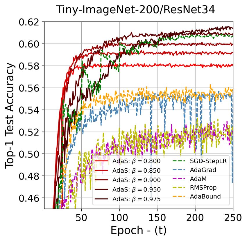
Under review as a conference paper at ICLR 2021

requires minimal hyper-parameter tuning effort. Despite the ease of implementation of such optimiz-
ers, there is a growing concern about their poor “generalization” characteristics. They perform well
on the given-samples i.e. training data, but perform poorly on the out-of-samples i.e. test/evaluation
data (Keskar et al., 2017; Wilson et al., 2017; Li et al., 2019; Yu & Zhu, 2020). In retrospect, the
non-adaptive SGD based optimizers (such as scheduled learning by Warmup Techniques Loshchilov
& Hutter (2017), Cyclical-Learning Smith (2017); Smith & Topin (2019), and Step-Decaying Good-
fellow et al. (2016)) are still dominantly used in training CNNs to achieve high performance at the
price of either more epochs for training and/or costly tuning for optimal hyper-parameter configura-
tions; given different datasets and models.
Unfortunately, such scheduling techniques are human-intuitive-based approaches. For instance, in
step-decaying method, the learning rate is suggested to start from a high value and then drop in
several epoch steps Goodfellow et al. (2016); Loshchilov & Hutter (2017), or it is suggested to
start from small value and increase as the epoch training proceeds to drop down again to finalize
training Smith (2017); Smith & Topin (2019). Unfortunately, there is little understood from such
methods why they should really work? It really becomes more like an alchemy rather than analyt-
ical/empirical reasoning. Recent investigations reveal that these two different scheduling scenario
actually cause different generalization characteristics Li et al. (2019). This simply creates a high
threshold for ML practitioners.
Our goal in this paper is twofold: (1) we introduce new probing metrics that enable the monitoring
of the well-posedness of learning layers in Convolution Neural Network (CNN); and (2) we pro-
pose a new learning function ψ and accordingly tailor an adaptive optimization algorithm. Unlike
the general trend where the raw gradients are used in ψ(·) for adapting the step-size (by some sort
of statistics measure), we avoid direct measuring of the gradients and associate this learning func-
tion with one of the proposed metrics called the “knowledge gain”. This gain is measured by the
energy norm of low-rank factorization of convolution weights which basically defines “the useful
knowledge carried over gradient updates”. Our main contributions are as follows.
Probing metrics. The concepts of “Knowledge Gain - (G)” and “Mapping Condition - (C)” are
introduced to quantify the well-posedness of convolutional layers. The gain G encodes the useful
information carried over each convolution layer and the condition C encodes the numerical stability
of feature mapping from input to the output layer. Using the probing metrics, we provide empirical
evidences on the generalization performance of different stochastic optimizers and explain how
different layers in CNN can function as a better autoencodeer over epoch training.
AdaS. A new adaptive optimizer is introduced by defining the learning function (that is independent
to each network layer) inversely proportional to the difference of knowledge gain over consecutive
epochs i.e. ψ(·) ∝ 1/[G(wt+1 ) − G(wt )]. We associate the final learning rate with a “gain fac-
tor - (β)” by exponential decaying average of learning functions over epoch training. The factor
trades-off between fast convergence and optimum performance which we leave it up to the user as a
preference choice to either save training time or reach to a maximum possible accuracy.
Experimentation. Thorough experiments are conducted in the context of image classification prob-
lem using various dataset and CNN models. The empirical results reveal that AdaS converges much
faster while maintaining superior generalization ability.

1.1   R ELATED W ORKS

The first adaptive optimizer was introduced in Duchi et al. (2011) (AdaGrad) by regulating the
update size with the accumulated second order statistical measures of gradients. The issue of van-
ishing learning rate caused by equally weighted accumulation of gradients is the main drawback of
AdaGrad that was raised in Tieleman & Hinton (2012) (RMSProp), which utilizes the exponential
decaying average of gradients instead of accumulation. A variant of first-order gradient measures
was also introduced in Zeiler (2012) (AdaDelta), which solves the decaying learning rate problem
using an accumulation window. The adaptive moment estimation in Kingma & Ba (2014) (Adam)
was introduced later to leverage both first and second moment measures of gradients. Adam solves
the vanishing learning rate problem and offers a more optimal adaptive learning rate to improve in
rapid convergence and generalization capabilities. Further improvements were made on Adam using
Nesterov Momentum Dozat (2016), long-term memory of past gradients Reddi et al. (2018), recti-
fied estimations Liu et al. (2020), dynamic bound of learning rate Luo et al. (2019), hyper-gradient

                                                  2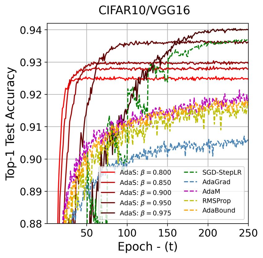
Under review as a conference paper at ICLR 2021

descent method Baydin et al. (2018), and loss-based step-size Rolinek & Martius (2018). Methods
based on line-search techniques Vaswani et al. (2019) and coin betting Orabona & Tommasi (2017)
are also introduced to avoid bottlenecks caused by the hyper-parameter tuning issues.

2     O N N EW M ETRIC M EASURE T OOLS
In this section we develop new metrics that can be probed in intermediate layers of CNN to measure
the well-posedness of each convolution layer. We first adopt the low-rank factorization for CNN.

2.1   L OW-R ANK FACTORIZATION OF C ONVOLUTION W EIGHTS

Consider the convolutional weights of a CNN layer defined by a four-way array (aka fourth-order
tensor) W ∈ RN1 ×N2 ×N3 ×N4 , where N1 and N2 are the height and width of the kernels, and N3
and N4 the input and output channel sizes, respectively. The feature mapping under this convo-
                               PN3
lution operates by FO :,:,i4 =
                                         I                             I     O
                                  i3 =1 F:,:,i3 ∗ W:,:,i3 ,i4 , where F and F are the input and output
feature maps (stacked in 3D volumes), and i4 ∈ {1, . . . , N4 } is the output index. The well-
posedness of this feature mapping can be studied by the generalized spectral decomposition (i.e.
SVD) of tensor arrays using the Tucker model Kolda & Bader (2009); Sidiropoulos et al. (2017)
      PN PN PN PN
W = i11=1 i22=1 i33=1 i44=1 Gi1 ,i2 ,i3 ,i4 ui1 } ui2 } ui3 } ui4 , where, the core G (containing
singular values) is called a (N1 , N2 , N3 , N4 )-tensor, uik ∈ RNk is the factor basis for decomposi-
tion, and } is outer product operation.
The weight structure W is initialized at random in CNN training where new structure will be learned
throughout iteration training lying in the tensor space; presumably in a mixture of a low-rank mani-
fold and perturbing noise. In fact, this is the main rationale behind many CNN compression methods
(such as in Lebedev et al. (2015); Tai et al. (2016); Kim et al. (2016); Yu et al. (2017)). This is mainly
done by factorizing the observing weights W = W+E,  b      where, W b corresponds to the low-rank tensor
pertinent to the small-core tonsor. A handful of techniques are deployed to approximate the small
core tensor by minimizing the error residues E = ||W − W||      b 2 Kolda & Bader (2009); Oseledets
                                                                    F
(2011); Grasedyck et al. (2013); Sidiropoulos et al. (2017). Most solutions, however, cast iterative
algorithms and create computation burden.
Here, we consider vector form vec (W) = (U1 ⊗ U2 ⊗ U3 ⊗ U4 ) vec (G), where vec (·) is a vector
obtained by stacking all tensor elements column-wise, ⊗ is the Kronecker product, and Ui is a
factor matrix containing all bases uik stacked in column. To decompose input and output channels
of convolution weights, we use mode-3 and mode-4 vector expressions
             W3 = (U1 ⊗ U2 ⊗ U4 ) G3 UT3 and W4 = (U1 ⊗ U2 ⊗ U3 ) G4 UT4 ,                      (2)
                N1 N2 N4 ×N3           N1 N2 N3 ×N4
where, W3 ∈ R                , W4 ∈ R               , and G3 and G4 are likewise reshaped forms of
the core tensor G. The vector decomposition in 2 is a two-way array (aka matrix) representation
e.g. W3 = U ΛV T where U ≡ U1 ⊗ U2 ⊗ U4 , V ≡ U3 , and Λ ≡ G3 Sidiropoulos et al.
(2017). In other words, to decompose a tensor on a given mode, the tensor is unfolded first and
                                                                 unfold        decompose
a decomposition of interest is applied (such as SVD) i.e. W −−−−→ W3 −−−−−−−→ U ΛV T .
The noise presence, however, prevents better understanding of the latter reshaped forms. Similar to
Lebedev et al. (2015), we revise our goal into low-rank matrix factorizations of W3 = W  c3 + E3
and W4 = W4 + E4 . The global analytical solution is given by the Variational Baysian Matrix
             c
Factorization (VBMF) technique in Nakajima et al. (2013) as a re-weighted SVD of the observation
matrix. This method avoids unnecessary implementing an iterative algorithm. Figures 4.2 and 1(b)
demonstrate the singular values obtained by decomposing multiple layers of VGG16 network.

2.2   W ELL -P OSED S TRUCTURE OF C ONVOLUTION W EIGHTS

At the core of our metric definition is the “well-posed” structure of convolution weights in CNN and
how they effect the casecade mapping of the features along the network layers. Recall the low-rank
factorization of a tensor weight to be decomposed by the following procedure
                           unfold                     Factorize c
             W (Tensor) −−−−→ Wd (2D-Matrix) −−−−−−−→ W             d (Low-Rank) + Ed .

                                                    3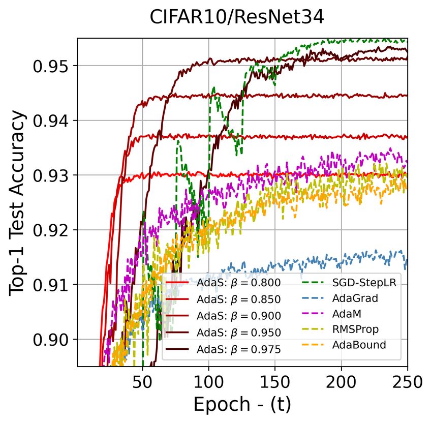
Under review as a conference paper at ICLR 2021
We importantly factorize Wd = W cd + Ed where Ed is some perturbing noise that we subsequently
ignore and Wd is a low-rank factorized matrix of Wd . In this formulation, the randomness of
c
initialization is captured by Ed and thus filtered when ignore it, and we apply SVD on the low-rank
factorized matrix W cd = U bd Λb d Vb T to determine the structural characteristics of the weights. We
d
refer to Λ
b d as being the singular values of the low-rank matrix. We now define the “well-posedness”
by
Pb
1. the summation of singular values Λ d should be high to guarantee the space-span (under
the convolution layer mapping) is mainly encoded by the low-rank structure, but not the
noise perturbation (aka the low-rank energy is dominant kW cd k
kEd k)
2. the relative ratio of the highest to the lowest singular values Λb max /Λb min should be low to
d d
guarantee the perturbation of feature-space (under the convolution layer mapping) is mainly
related to the noise sampling but not the low-rank structure
Under the above assumptions, one can claim that the feature mapping by the convolution layer can
pose a meaningful structure for feature decomposition i.e. layers can better fit the training data.
2.3 D EFINING M ETRICS
Following the conditions of well-posed structure, we introduce the following two definitions.
Definition 1. (Knowledge Gain–G). The knowledge gain across a particular channel (dth dimen-
sion) of a layer in CNN is defined by
0
Nd
1 X
Gdp (W) = σkp (W
cd ), (3)
Nd σ1p (W
cd )
k=1
where, σ1 ≥ σ2 ≥ · · · ≥ σNd0 are the low-rank singular values of a single-channel convolutional
weight in descending order, N 0 = rank W
cd , and p ∈ {1, 2}.
d
The remark of the Definition 1 is given in subsection A.3. The knowledge gain is a direct measure
of the normalized energy of low-rank structure of convolution weights. The division factor Nd in
(3) normalizes the gain G p ∈ [0, 1] as a fraction of channel capacity. The definition in Equation 3
is closely related to the stable-rank defined in Rudelson & Vershynin (2007). Note that we apply
Gd on channels d = {3, 4} (but not kernel size i.e. d = {1, 2}) to measure the gain through
input/output feature mapping. Figure 1(c) demonstrates the distribution of knowledge gain cross
all ResNet18 convolution layers trained on ImageNet. Throughout many experimental setup, we
noticed a consistent behavior where the knowledge gain of early layers are statistically significant
compared to the proceeding layers.
3 3 1 14
2.5 Conv Layer: 5 2.5 Conv Layer: 5
Conv Layer: 12 Conv Layer: 12 12
2 2 0.8
Mapping Condition
Conv Layer: 15 Conv Layer: 15
Knowledge Gain
Conv Layer: 17 Conv Layer: 17
10
Energy - ( )
Energy - ( )
1.5 1.5
Conv Layer: 19 Conv Layer: 19 0.6 8
1 1 6
0.4
4
0.2
2
0.5 0.5
0 0
100 200 300 400 500 100 200 300 400 500 5 10 15 20 5 10 15 20
Singular Value index Singular Value index Conv Index Conv Index
(a) Mode-3 Decomposition (b) Mode-4 Decomposition (c) 1
G4 (WResNet18 ) (d) C4 (WResNet18 )
Figure 1: Metric measurements using low-rank factorization of convolution weights from ResNet18
trained on ImageNet. Distribution of singular values are shown for (a) input channel and (b) output
channel; on multiple convolution layers of ResNet18. The solid and dashed lines correspond to with
and without low-rank factorization. The metrics of knowledge gain and mapping condition are also
shown in (c) and (d) cross all conv layers of ResNet18, respectively.
Definition 2. (Mapping Condition–C). The mapping condition across a particular channel (dth
dimension) of a layer in CNN is defined by
Cd (W) = σ1 (W
cd )/σN 0 (W
d
cd ), (4)
4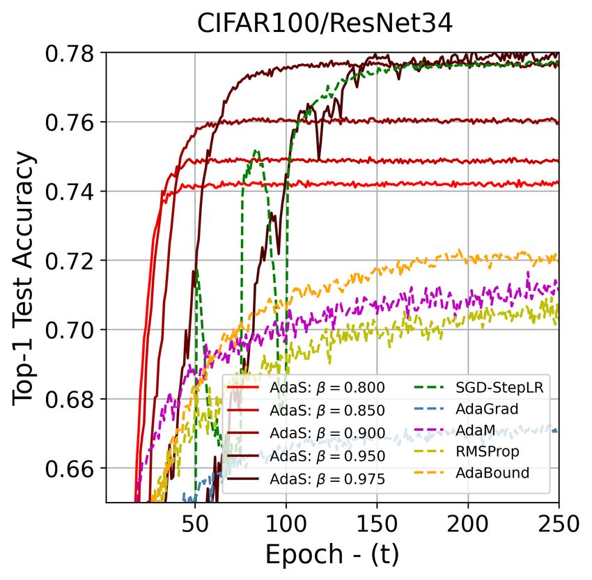
Under review as a conference paper at ICLR 2021

where, σ1 and σNd0 are the maximum and minimum low-rank singular values of a single-channel
convolutional weight, respectively.

The notion of mapping condition in Definition 2 is adopted from the matrix analysis theory Horn &
Johnson (2012) where it measures the relative ratio of maximum to minimum low-rank singular val-
ues. The number indicates the sensitivity of convolution mapping with respect to minor input pertur-
bations. High condition number pertains to poor stability and vice versa. Figure 1(d) demonstrates
the distribution of mapping condition cross all ResNet18 convolution layers trained on ImageNet.

3     L EARNING F UNCTION ψ(·) BY K NOWLEDGE G AIN
Our goal here is to motivate and introduce a new learning function ψ(·) for SGD update in (1). Recall
the convolution weight training in deep CNN Bottou (2010; 2012); Loizou & Richtárik (2020),
where the objective is to minimize an associated loss function given a train dataset f (W ; (X)train ).
The update rule for SGD minimization therefore is given by
              W k ←− W k−1 − ηk ∇f k (W k−1 ) for k ∈ {(t − 1)K + 1, · · · , tK},                      (5)
where, t and K correspond         to epoch index and number of mini-batches, respectively,
∇f k (W k−1 ) = 1/|Ωk | i∈Ωk ∇fi (W k−1 ) is the average stochastic gradients on kth mini-batch
                         P

that are randomly selected from a batch of n-samples Ωk ⊂ {1, · · · , n}, and ηk defines the step-size
taken toward the opposite direction of average gradients.
We aim to update the learning function once at each epoch and therefore the step-size will be a
function of epoch index i.e. ηk ≡ η(t). We now setup our problem by accumulating all observed
gradients throughout K mini-batch updates fit in one epoch training
                                     W t = W t−1 − η(t − 1)∇f t ,                                      (6)
                PtK
where, ∇f t = k=(t−1)K+1 ∇f k (W k−1 ) corresponds to the total accumulated gradients in one
epoch training. The idea here is to select a learning rate η(t) such that knowledge gain from one
epoch training to another is increased i.e. ψ = {η(t) : G(W t ) ≥ G(W t−1 )}. Why is that?
From the definition of knowledge gain in previous section, higher G(W ) corresponds to a better en-
coder such that the index of separability will be increased for better space spanning via convolution
mapping. Here we provide a satisfying conditions on the step-size.
Theorem 1. (Increasing Knowledge Gain for Vanilla SGD). Let the knowledge gain to be defined
by Equation 3. Starting with an initial learning rate η(0) > 0 and by setting the step-size of vanilla
Stochastic Gradient Descent (SGD) proportionate to
                                  η(t) , ζ G(W t ) − G(W t−1 )

                                                                                                   (7)
will guarantee the monotonic increase of the knowledge gain over consecutive epoch updates i.e.
G(W t+1 ) ≥ G(W t ) for some existing lower bound η(t) ≥ η0 and ζ ≥ 0.

The proof of Theorem 1 is provided in the Appendix A.
Note that with the start of a positive initial learning rate η(0) > 0 and following the update rule in (7),
Theorem 1 guarantees the increase of the knowledge gain for the next epoch update. Accordingly,
the positivity of learning rates using (7) will be maintained throughout consecutive epoch updates.

4     A DA S A LGORITHM
In this section, we introduce our scheduling algorithm AdaS for adaptive adjustment of learning-rate
adopted within the mSGD framework.

4.1   L EARNING R ATE BY E XPONENTIAL D ECAY AVERAGING (G AIN FACTOR β)

The step-size defined in 7 for vanilla SGD is only measured from two consecutive epochs i.e. t − 1
and t. Due to the stochastic nature of gradients, the increase of knowledge gain over two epochs

                                                    5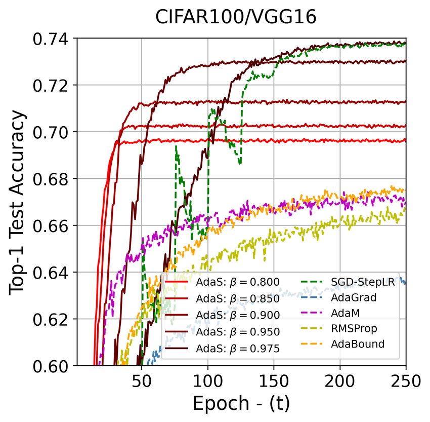
Under review as a conference paper at ICLR 2021

can fluctuate. To adapt a smooth change of learning-rate, we employ a momentum algorithm for
historic accumulation of step-sizes over epoch updates. The concept is similar to AdaM but with
only the difference where the updates are done at every epoch (not every mini-batch). It also worth
noting that this is different from the momentum update in SGD (mSGD) where the gradients are
accumulated over mini-batch updates i.e. k.
We formulate the update rule for AdaS using the mSGD framework as follows
      -update learning rate with momentum: η(t, `) ← βη(t − 1, `) + ζ[G(t, `) − G(t − 1, `)],
      -update gradients with momentum: v`k ← αv`k−1 − η(t, `)g`k ,                                    (8)
      -weights update: w`k ← w`k−1 + v`k ,
where, k is the current mini-batch iteration, t is the current epoch, ` is the conv block index, G(·) is
the average knowledge gain obtained from both input and output channels of convolution layers, v
is the velocity term, and w are the learnable parameters. Notice there are two associated momentum
parameters: gradient momentum adopted from mSGD fixed at default rate α = 0.9, and learning
rate momentum β which we call it the “gain factor”. Setting this parameter trades-off between
faster convergence and increased performance. This is up to the user to select and it will impact the
final performance and training time e.g. β = 0.8 takes ≈ 50 epochs (4.86 hours) for Tiny-ImageNet
to train and converge, while for β = 0.9 this consumes twice the number of epochs ≈ 100 to
converge with higher performance. An ablative study on the effect of this parameter is provided in
Experiment Section 5.1 as well as in the Appendix-BD. Note that we fix ζ = 1 for all experiments in
this paper as it becomes a redundant parameter since the relative ratio of learning rate is now directly
controlled by β.

Algorithm 1: Adaptive Scheduling (AdaS) for mSGD
                                                                                             L
Require       : batch size n, # of epochs T , # of conv blocks L, initial step-sizes {η(0, `)}`=1 ,
                                                L                                    L
                initial momentum vectors v`0 `=1 , initial parameter vectors w`0 `=1 , mSGD
                momentum rate α = 0.9, AdaS gain factor β ∈ [0, 1).
for t = 1 : T do
    // Phase-I: mSGD optimization by adaptive learning rates
    randomly shuffle dataset, generate K mini-batches {Ωk ⊂ {1, · · · , n}}K   k=1
    for k = (t − 1)K + 1 : tK do
        1. compute gradient: g`k ← 1/|Ωk | i∈Ωk ∇fi (w`k−1 ), ` ∈ {1, · · · , L}
                                              P

        2. compute the velocity term: v`k ← αv`k−1 − η(t, `)g`k
        3. apply update: w`k ← w`k−1 + v`k
    end
    // Phase-II: adaptive computation of learning rates
    for ` = 1 : L do
        1. unfold tensors using (2): Wd ← mode-d Wt` for d = {3, 4}


        2. factorize low-ranks Nakajima et al. (2013): W cd ← EVBMF (Wd ) for d = {3, 4}
        3. compute average knowledge gain using (3): G(t, `) ← [G31 (W) + G41 (W)]/2
        4. compute learning rate momentum:
         η(t + 1, `) ← βη(t − 1, `) + [G(t, `) − G(t − 1, `)]
        5. lower bound the learning rate: η(t + 1, `) ← max (η(t + 1, `), 0)
    end
end

4.2     A LGORITHM

The pseudo-code for our proposed algorithm AdaS is presented in Algorithm 1. Each convolution
block in CNN is assigned with an index {`}L   `=1 where all learnable parameters (e.g. conv, biases,
batch-norms, etc) are called using this index. The goal in AdaS is firstly to callback the convolution
weights of each layer, secondly compute the overall knowledge gain G(t, `) of each layer using (3),
thirdly compute the difference gain using (7), and finally accumulate this difference value in expo-
nential decay averaging (as discussed in previous section) to compute the associated learning rate of
current epoch t to plug in the mSGD optimization framework. We note here that the initial knowl-

                                                   6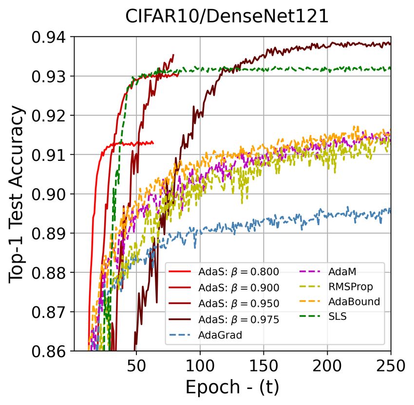
Under review as a conference paper at ICLR 2021

edge gain yields zero G(0, `) = 0 for all conv layers due to random initialization of weights. Figure
2 (left plot) demonstrates an evolution example of the learning rate adapted by AdaS algorithm. In-
terestingly, the behavior of learning rate coincides with cyclical learning scheduling in Smith (2017);
Smith & Topin (2019). We believe our method explains the intuition behind such scheduling tech-
nique that why the rate is suggested to start with small rate → increase with proceeding epochs →
and then decrease to finalize training.

Figure 2: Metric evaluation of two different optimizers: AdaSβ=0.8 and AdaM. Both average knowl-
edge gain G(t, `) and average mapping condition C(t, `) are monitored for duration of all epoch
training of VGG16 on CIFAR10. The evolution of learning rate η(t) are also shown in left. The
plots with different color shades correspond to multiple layers of the network.

Here we provide the convergence rate for AdaS.
Theorem 2. (AdaS convergance [adopted from Loizou & Richtárik (2020)]). Let {wk }k=0  ∞    be
the random sequence generated by AdaS algorithm in 1, and w∗ be the converging point. Assume
0 ≤ η(t) < 2 and α ≥ 0, and the expressions a1 (t) , 1+3α+2α2 −(η(t)(2 − η(t)) + αη(t)) λ+ min
and a2 (t) , α + 2α2 + αη(t)λmax satisfy a1 (t) + a2 (t) < 1. Then the convergence rate of the
generated sequences is bounded by
                       E kwk − w∗ k2B ≤ q(t)k (1 + δ(t))kw0 − w∗ k2B ,

                                                                                           (9)
and the convergence rate of the loss function is bounded by
                        E f (wk ) ≤ q(t)k λmax                      ∗ 2
                                                            0
                                                2 (1 + δ(t))kw − w kB ,
                                                                                              (10)
                        p
                             2
 where, q(t) = (a1 (t) + a1 (t) + 4a2 (t))/2 and δ(t) = q(t) − a1 (t). Moreover, a1 (t) + a2 (t) ≤
q(t) < 1.
Theorem 2 is mainly adopted from Loizou & Richtárik (2020) to analyze mSGD convergence. The
update rule in AdaS in fact introduces minor adjustments to the proof which we describe in Appendix
A.2. Following the convergence rate in (9), within one training epoch, AdaS enjoys the convergence
rule of the fixed learning rate, 0 < η < 2 in mSGD. Further, the learning rate under AdaS continues
to decreases, contracting the convergence rate in (9) i.e. q(t)k (1 + δ(t)) decays quicker as the
learning rate η(t) decreases over epoch progression and hence yields a faster speed for training.
Empirical Reasoning on Generalization Ability of Optimizers. In Figure 2, the performance
of AdaS optimizer is compared to AdaM by monitoring the evolution of both metrics of knowledge
gain and mapping condition on multiple layers of CNN. Both optimizers gain knowledge over epoch
training where the gain for early layers of network yield relatively higher value compared to the
proceeding layers. We relate this to better encoding capability of the network in early stage of conv
layers. We also make an extra interesting observation where AdaS yields much lower mapping
condition in different conv layers (shown in different colors) as opposed to AdaM. Particularly,
the last layers of AdaM yield much higher condition number. We relate this phenomena to poor
generalization of AdaM. For more experimentation, please refer to Appendix D.
AdaS Computational Overhead. Note that AdaS uses mSGD’s framework for adapting the learing
rates. The computational overhead introduces by AdaS is only related to the low-rank factorization
per epoch update using EVBMF method introduced in phase-II of the algorithm 1. The factorization
use quadratic minimization for matrix decomposition which is linear to the matrix size. AdaS easily
scales to many CNN models for optimization. In comparison, the adaptive optimizers such as Adam
use different statistical model per mini-batch training where the computational overhead is very well
comparable with AdaS. For instance, all mSGD+StepLR, AdaS, AdaM, RMSProp, AdaBound, and
AdaGrad consume ∼ 40 min per epoch to train ResNet34 on ImageNet using the experimental setup
defined in Appendix B.

                                                  7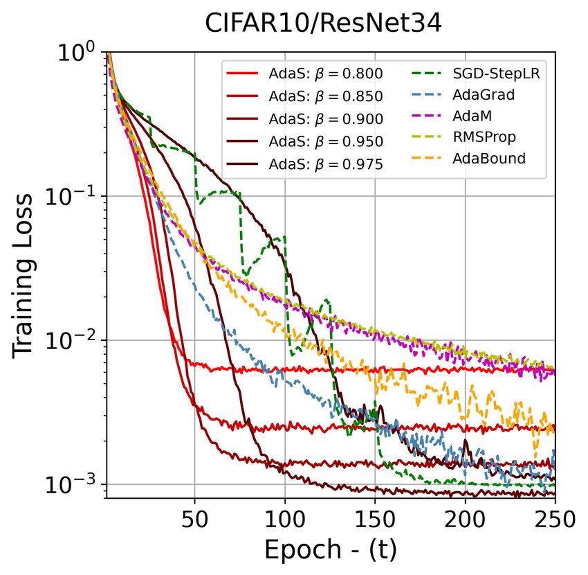
Under review as a conference paper at ICLR 2021
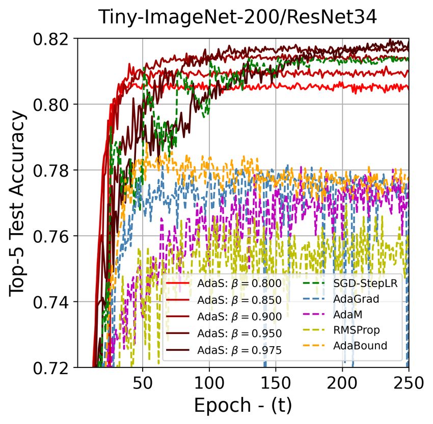
Figure 3: Training performance using different optimizers across three different datasets (i.e. CI-
FAR10, CIFAR100, Tiny-ImageNet-200) and two different CNNs (i.e. VGG16 and ResNet34).
5 E XPERIMENTS
We compare our AdaS algorithm to several adaptive optimizers in the context of image classifi-
cation. In particular, we implement AdaGrad Duchi et al. (2011), RMSProp Goodfellow et al.
(2016), AdaM Kingma & Ba (2014), AdaBound Luo et al. (2019), and SLS Vaswani et al. (2019)
for comparison. We also implement mSGD-StepLR guided by scheduled dropping (step decaying)
Goodfellow et al. (2016) to understand the baseline for achieving high accuracy that is extensively
used in the literature for training CNNs. We further investigate the efficacy of AdaS with respect to
variations in the number of deep layers using VGG16 Simonyan & Zisserman (2015), ResNet18 and
ResNet34 He et al. (2016), ResNeXt50 Xie et al. (2017), and DenseNet121 Huang et al. (2017), and
the number of class datasets using the standard CIFAR-10 and CIFAR-100 Krizhevsky et al. (2009),
Tiny-ImageNet-200 (Li et al.), and ImageNet Russakovsky et al. (2015) for training. Please refer
to Appendix B for details of experimental setup, Appendix C for additional experiments, as well as
Appendix D for AdaS ablative studies.
5.1 R ESULTS
Generalization Performance. The primary results of each experiment are visualized in Figure 3
(additional results are also shown in Figure 6 in Appendix D). The experiments demonstrate how
well our optimizer AdaS is generalized across different dataset and network. AdaS, with low gain
factors (e.g. β = 0.8), consistently outperforms all other adaptive optimizers in terms of conver-
gence speed, as well as achieving superior test accuracy. For instance, AdaSβ=0.8 outperforms
AdaM in CIFAR100/ResNet34 with ∼ 5.5% improvement in test accuracy; within 50 epoch train-
ing. Also, both SGD-StepLR and AdaS (with higher β) eventually overtake the other methods; once
enough epochs are trained. The overall generalization of SGD-StepLR however is inferior to AdaS
(using high β) where AdaS yields faster convergence to achieve high accuracies; at times even bet-
ter than SGD-StepLR e.g. Tiny-ImageNet-200/ResNet34, CIFAR10/VGG16, CIFAR100/VGG16,
and CIFAR100/ResNet34 (see also Table 1 for tabulated results). All optimizers achieve low training
losses/training accuracies, but do not exhibit equivalently to high test accuracies. Such inconsistency
is more evident for adaptive optimizers i.e. AdaGrad, RMSProp, AdaM, and AdaBound. Such poor
8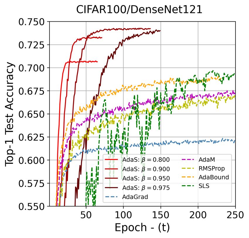
Under review as a conference paper at ICLR 2021

generalization coincides with the reports made in Wilson et al. (2017); Li et al. (2019); Jastrzebski
et al. (2020) where adaptive optimizers generalize worse compared to non-adaptive methods.
On Fixed Epoch-Budget Performance. We further provide quantitative results on the convergence
of all optimizers trained on ResNet34 in Table 1 with fixed number of epochs. The rank consistency
of AdaS (using low/high β) over other optimizers is evident. For instance, AdaSβ=0.80 gains 11.63%
test accuracy improvement over AdaM optimizer on Tiny-ImageNet-200 trained withing 50 epochs.

Table 1: Image classification performance (test accuracy) of ResNet34 on CIFAR-10, CIFAR-100,
and Tiny-ImageNet-200 with fixed budget epochs. Three adaptive (AdaBound, AdaM, AdaS) and
one non-adaptive (SGD-StepLR) optimizers are deployed for comparison.
                                Epoch    AdaBound       AdaM      SGD-StepLR   AdaSβ=0.8     AdaSβ=0.9   AdaSβ=0.975
                                  50    90.84±0.17   91.54±0.35   86.53±1.67   93.04±0.13   94.35±0.22   88.91±1.30
        CIFAR-10

                                 100    92.03±0.44   92.71±0.27   92.25±0.29   93.03±0.16   94.48±0.13   93.09±0.52
                                 150    92.67±0.14   93.07±0.33   94.64±0.09   93.00±0.17   94.45±0.11   94.99±0.23
                                 200    92.59±0.13   93.17±0.30   95.44±0.10   93.02±0.16   94.47±0.13   95.14±0.34
                                 250    92.74±0.16   93.22±0.36   95.43±0.08   93.02±0.13   94.46±0.12   95.24±0.15
                                  50    68.02±0.75   68.66±0.46   62.17±1.68   74.18±0.32   75.64±0.25   62.49±1.60
      Tiny-ImageNet CIFAR-100

                                 100    70.57±0.40   69.78±0.27   68.78±0.97   74.21±0.35   76.02±0.10   74.48±0.53
                                 150    71.67±0.49   70.45±0.42   77.40±0.46   74.22±0.35   76.00±0.13   77.81±0.23
                                 200    72.08±0.27   70.61±0.33   77.63±0.42   74.19±0.24   76.05±0.11   77.76±0.38
                                 250    71.94±0.66   71.11±0.37   77.65±0.32   74.21±0.26   75.99±0.09   78.00±0.28
                                  50    54.15±1.13   47.43±1.60   53.03±1.55   57.85±0.55   58.95±0.45   55.19±0.74
                                 100    55.37±0.15   48.97±1.86   57.99±0.38   58.06±0.48   59.97±0.33   59.19±0.49
                                 150    55.00±0.85   52.22±0.51   59.99±0.27   57.99±0.36   59.97±0.40   60.22±0.27
                                 200    55.05±0.58   50.14±1.20   60.59±0.49   58.16±0.40   60.01±0.30   61.13±0.37
                                 250    55.48±0.67   52.13±1.14   60.65±0.39   57.98±0.44   59.91±0.45   61.44±0.27

Note that for a given fixed epoch budget, one might tune the initial learning rates, as well as the
other hyper-parameters (such as weight-decay, batch-size, momentum, etc) to achieve optimum per-
formance accuracy. However, this comes with a huge price of tuning effort that is required by the
end-user. Therefore, providing a fast converging optimizer such as AdaS (with minimal tuning
effort) is imperative to achieve high performing accuracy.
Is β a hyper-parameter to tune? β (gain factor) is not a hyper-parameter but a design choice for
application. Considering the computational budget, the gain offers to either (a) tune for “Speedy
Convergence” by setting it low e.g. β = 0.8, or (b) tune for “Greedy Convergence” by setting it
high e.g. β = 0.975. The selection of different β directly translates to different number of epoch
trains. The speedy convergence is set to train rapidly with minimal sacrifice on the accuracy–AdaS
performs much better than all adaptive optimizers in terms of accuracy and speed which is highly
desirable in many optimization methods such as neural architecture search. The greedy convergence
case can also be used to achieve maximum possible accuracy, similar to mSGD-StepLR, assuming
the computational budget is unlimited.

6   C ONCLUSION

We proposed two new metrics to prob in the intermediate layers of CNN and define the well-
posedness of convolution layers. The metrics can be used alone for empirical reasoning of network
generalization performance. Provided by one of the metrics, we tailor a new adaptive optimizer
AdaS to define learning rate of mSGD as a function of relative metric change over consecutive
epoch training. The optimizer admits super convergence characteristics as well as high generaliza-
tion performance compared to many adaptive and non-adaptive optimizers. We highlight that these
improvements come through the application of AdaS to simple mSGD. We further identify that since
AdaS adaptively tunes the learning rates, it can be deployed with optimizers such as AdaM, replac-
ing the traditional scheduling techniques. Finally, this paper only studied optimization for CNNs
and we will extend this to the general form of DNNs for future work.

R EFERENCES
Atilim Gunes Baydin, Robert Cornish, David Martinez Rubio, Mark Schmidt, and Frank Wood. On-
  line learning rate adaptation with hypergradient descent. In International Conference on Learning

                                                                       9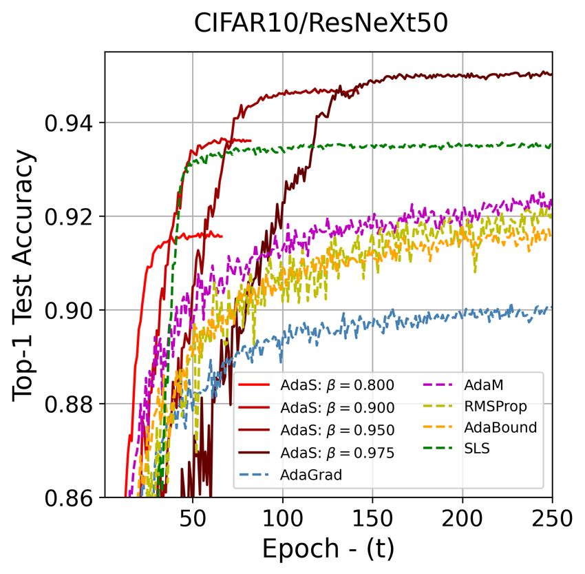
Under review as a conference paper at ICLR 2021

  Representations, 2018. URL https://openreview.net/forum?id=BkrsAzWAb.
Yoshua Bengio. Practical recommendations for gradient-based training of deep architectures. In
  Neural networks: Tricks of the trade, pp. 437–478. Springer, 2012.
Léon Bottou. Large-scale machine learning with stochastic gradient descent. In Proceedings of
   COMPSTAT’2010, pp. 177–186. Springer, 2010.
Léon Bottou. Stochastic gradient descent tricks. In Neural networks: Tricks of the trade, pp. 421–
   436. Springer, 2012.
Didier A Depireux, Jonathan Z Simon, David J Klein, and Shihab A Shamma. Spectro-temporal
  response field characterization with dynamic ripples in ferret primary auditory cortex. Journal of
  neurophysiology, 85(3):1220–1234, 2001.
Timothy Dozat. Incorporating nesterov momentum into adam. 2016.
John Duchi, Elad Hazan, and Yoram Singer. Adaptive subgradient methods for online learning and
  stochastic optimization. Journal of Machine Learning Research, 12(61):2121–2159, 2011. URL
  http://jmlr.org/papers/v12/duchi11a.html.
Ian Goodfellow, Yoshua Bengio, and Aaron Courville. Deep learning. MIT press, Cambridge, MA,
  USA, 2016. http://www.deeplearningbook.org.
Lars Grasedyck, Daniel Kressner, and Christine Tobler. A literature survey of low-rank tensor
  approximation techniques. GAMM-Mitteilungen, 36(1):53–78, 2013.
Kaiming He, Xiangyu Zhang, Shaoqing Ren, and Jian Sun. Deep residual learning for image recog-
  nition. In Proceedings of the IEEE conference on computer vision and pattern recognition, pp.
  770–778, 2016.
Roger A Horn and Charles R Johnson. Matrix analysis. Cambridge university press, 2012.
Gao Huang, Zhuang Liu, Laurens Van Der Maaten, and Kilian Q Weinberger. Densely connected
  convolutional networks. In Proceedings of the IEEE conference on computer vision and pattern
  recognition, pp. 4700–4708, 2017.
Stanislaw Jastrzebski, Maciej Szymczak, Stanislav Fort, Devansh Arpit, Jacek Tabor, Kyunghyun
  Cho*, and Krzysztof Geras*. The break-even point on optimization trajectories of deep neural
  networks. In International Conference on Learning Representations, 2020. URL https://
  openreview.net/forum?id=r1g87C4KwB.
Nitish Shirish Keskar, Dheevatsa Mudigere, Jorge Nocedal, Mikhail Smelyanskiy, and Ping Tak Pe-
  ter Tang. On large-batch training for deep learning: Generalization gap and sharp minima. In
  International Conference on Learning Representations, 2017. URL https://openreview.
  net/forum?id=H1oyRlYgg.
Yong-Deok Kim, Eunhyeok Park, Sungjoo Yoo, Taelim Choi, Lu Yang, and Dongjun Shin. ompres-
  sion of deep convolutional neural networks for fast and low power mobile applications. jan 2016.
  4th International Conference on Learning Representations, ICLR 2016.
Diederik P Kingma and Jimmy Ba. Adam: A method for stochastic optimization. arXiv preprint
  arXiv:1412.6980, 2014.
Tamara G Kolda and Brett W Bader. Tensor decompositions and applications. SIAM review, 51(3):
  455–500, 2009.
Alex Krizhevsky, Geoffrey Hinton, et al. Learning multiple layers of features from tiny images.
  2009.
Vadim Lebedev, Yaroslav Ganin, Maksim Rakhuba, Ivan Oseledets, and Victor Lempitsky.
  Speeding-up convolutional neural networks using fine-tuned cp-decomposition. jan 2015. 3rd
  International Conference on Learning Representations, ICLR 2015.

                                                10
Under review as a conference paper at ICLR 2021
Yann LeCun, Yoshua Bengio, and Geoffrey Hinton. Deep learning. nature, 521(7553):436–444,
2015.
Fei-Fei Li, Andrej Karpathy, and Justin Johnson. URL https://tiny-imagenet.
herokuapp.com/.
Yuanzhi Li, Colin Wei, and Tengyu Ma. Towards explaining the regularization effect of initial large
learning rate in training neural networks. In Advances in Neural Information Processing Systems,
pp. 11674–11685, 2019.
Liyuan Liu, Haoming Jiang, Pengcheng He, Weizhu Chen, Xiaodong Liu, Jianfeng Gao, and Ji-
awei Han. On the variance of the adaptive learning rate and beyond. In International Confer-
ence on Learning Representations, 2020. URL https://openreview.net/forum?id=
rkgz2aEKDr.
Nicolas Loizou and Peter Richtárik. Momentum and stochastic momentum for stochastic gradi-
ent, newton, proximal point and subspace descent methods. Computational Optimization and
Applications, pp. 1–58, 2020.
Ilya Loshchilov and Frank Hutter. Sgdr: Stochastic gradient descent with warm restarts. 2017. 5th
International Conference on Learning Representations, ICLR 2017.
Liangchen Luo, Yuanhao Xiong, and Yan Liu. Adaptive gradient methods with dynamic bound of
learning rate. In International Conference on Learning Representations, 2019. URL https:
//openreview.net/forum?id=Bkg3g2R9FX.
Shinichi Nakajima, Masashi Sugiyama, S Derin Babacan, and Ryota Tomioka. Global analytic
solution of fully-observed variational bayesian matrix factorization. Journal of Machine Learning
Research, 14(Jan):1–37, 2013.
Francesco Orabona and Tatiana Tommasi. Training deep networks without learning rates through
coin betting. In Advances in Neural Information Processing Systems, pp. 2160–2170, 2017.
Ivan V Oseledets. Tensor-train decomposition. SIAM Journal on Scientific Computing, 33(5):2295–
2317, 2011.
Boris Polyak. Some methods of speeding up the convergence of iteration methods. Ussr Compu-
tational Mathematics and Mathematical Physics, 4:1–17, 12 1964. doi: 10.1016/0041-5553(64)
90137-5.
Sashank J. Reddi, Satyen Kale, and Sanjiv Kumar. On the convergence of adam and beyond. In
International Conference on Learning Representations, 2018. URL https://openreview.
net/forum?id=ryQu7f-RZ.
Herbert Robbins and Sutton Monro. A stochastic approximation method. The annals of mathemati-
cal statistics, pp. 400–407, 1951.
Michal Rolinek and Georg Martius. L4: Practical loss-based stepsize adaptation for deep learning.
In Advances in Neural Information Processing Systems, pp. 6433–6443, 2018.
Mark Rudelson and Roman Vershynin. Sampling from large matrices: An approach through geo-
metric functional analysis. Journal of the ACM (JACM), 54(4):21–es, 2007.
Olga Russakovsky, Jia Deng, Hao Su, Jonathan Krause, Sanjeev Satheesh, Sean Ma, Zhiheng
Huang, Andrej Karpathy, Aditya Khosla, Michael Bernstein, et al. Imagenet large scale visual
recognition challenge. International journal of computer vision, 115(3):211–252, 2015.
Tom Schaul, Sixin Zhang, and Yann LeCun. No more pesky learning rates. In International Con-
ference on Machine Learning, pp. 343–351, 2013.
Nicholas D Sidiropoulos, Lieven De Lathauwer, Xiao Fu, Kejun Huang, Evangelos E Papalexakis,
and Christos Faloutsos. Tensor decomposition for signal processing and machine learning. IEEE
Transactions on Signal Processing, 65(13):3551–3582, 2017.
11Under review as a conference paper at ICLR 2021
K. Simonyan and A. Zisserman. Very deep convolutional networks for large-scale image recogni-
tion. In International Conference on Learning Representations, 2015.
Leslie N Smith. Cyclical learning rates for training neural networks. In 2017 IEEE Winter Confer-
ence on Applications of Computer Vision (WACV), pp. 464–472. IEEE, 2017.
Leslie N Smith and Nicholay Topin. Super-convergence: Very fast training of neural networks using
large learning rates. In Artificial Intelligence and Machine Learning for Multi-Domain Operations
Applications, volume 11006, pp. 1100612. International Society for Optics and Photonics, 2019.
Ilya Sutskever, James Martens, George Dahl, and Geoffrey Hinton. On the importance of initial-
ization and momentum in deep learning. In International conference on machine learning, pp.
1139–1147, 2013.
Cheng Tai, Tong Xiao, Yi Zhang, Xiaogang Wang, and E. Weinan. Convolutional neural networks
with low-rank regularization. jan 2016. 4th International Conference on Learning Representa-
tions, ICLR 2016.
Tijmen Tieleman and Geoffrey Hinton. Lecture 6.5-rmsprop: Divide the gradient by a running
average of its recent magnitude. COURSERA: Neural networks for machine learning, 4(2):26–
31, 2012.
Sharan Vaswani, Aaron Mishkin, Issam Laradji, Mark Schmidt, Gauthier Gidel, and Simon Lacoste-
Julien. Painless stochastic gradient: Interpolation, line-search, and convergence rates. In Ad-
vances in Neural Information Processing Systems, pp. 3727–3740, 2019.
Ashia C Wilson, Rebecca Roelofs, Mitchell Stern, Nati Srebro, and Benjamin Recht. The marginal
value of adaptive gradient methods in machine learning. In Advances in Neural Information
Processing Systems, pp. 4148–4158, 2017.
Saining Xie, Ross Girshick, Piotr Dollár, Zhuowen Tu, and Kaiming He. Aggregated residual trans-
formations for deep neural networks. In Proceedings of the IEEE conference on computer vision
and pattern recognition, pp. 1492–1500, 2017.
Tong Yu and Hong Zhu. Hyper-parameter optimization: A review of algorithms and applications.
arXiv preprint arXiv:2003.05689, 2020.
Xiyu Yu, Tongliang Liu, Xinchao Wang, and Dacheng Tao. On compressing deep models by low
rank and sparse decomposition. In Proceedings of the IEEE Conference on Computer Vision and
Pattern Recognition, pp. 7370–7379, 2017.
Kun Yuan, Bicheng Ying, and Ali H Sayed. On the influence of momentum acceleration on online
learning. The Journal of Machine Learning Research, 17(1):6602–6667, 2016.
Matthew D Zeiler. Adadelta: an adaptive learning rate method. arXiv preprint arXiv:1212.5701,
2012.
A A PPENDIX -A: P ROOF OF T HEOREMS AND R EMARKS
A.1 P ROOFS FOR T HEOREM 1
The following two proofs correspond to the proof of Theorem 1 for p = 2 and p = 1, respectively.
Proof. (Theorem 1 for p = 2) Using the Definition 1, the knowledge gain of matrix W t+1 (assumed
to be a column matrix N ≤ M ) is expressed by
N0
t+1 1 X 1 T
G(W )= 2 t+1
σi2 (W t+1 ) = t+1 2 tr W t+1 W t+1 . (11)
N σ1 (W ) i=1 N ||W ||2
12Under review as a conference paper at ICLR 2021
An upper-bound of first singular value can be calculated by first recalling its equivalence to `2 -norm
and then applying the Cauchy–Schwarz inequality
σ12 (W t+1 ) = ||W t+1 ||22 = ||W t −η(t)∇f t+1 ||22 ≤ ||W t ||22 +η 2 (t)||∇f t+1 ||22 +2η(t)||W t ||2 ||∇f t+1 ||2 .
(12)
Note that η(t) is given by previous epoch update and considered to be positive (we start with an
initial learning rate η(0) > 0). Therefore, the right-hand-side of the inequality in (12) will be
positive and holds.
By substituting (12) in (11) and expanding the terms in trace, a lower bound of W t+1 is given by
1 h T T T
i
G(W t+1 ) ≥ tr W t W t − 2η(t) tr W t ∇f t+1 + η 2 (t) tr ∇f t+1 ∇f t+1 , (13)
Nγ
where, γ = ||W t ||22 + η 2 (t)||∇f t+1 ||22 + 2η(t)||W t ||2 ||∇f t+1 ||2 . The latter inequality can be
revised to
h
T
G(W t+1 ) ≥ N1γ 1 − ||Wγt ||2 + ||Wγt ||2 tr W t W t
2 2 i
T T
−2η(t) tr W t ∇f t+1 + η 2 (t) tr ∇f t+1 ∇f t+1
h
1 γ T γ T
= Nγ ||W t ||22
tr W t W t + 1 − ||W t ||22
tr W t W t
T
i
T
−2η(t) tr W t ∇f t+1 + η 2 (t) tr ∇f t+1 ∇f t+1
γ T T T
tr W t W t − 2η(t) tr W t ∇f t+1 + η 2 (t) tr ∇f t+1 ∇f t+1
1
= G(W t ) + 1−
.
Nγ ||W t ||22
| {z }
D
(14)
Therefore, the bound in (14) is revised to
1
G(W t+1 ) − G(W t ) ≥ D. (15)
Nγ
Since γ ≥ 0, the monotonicity of the Equation (15) is guaranteed if D ≥ 0. The remaining term D
can be expressed as a quadratic function of η
||22
h T
i
||∇f tT t
D(η) = tr ∇f t+1 ∇f t+1 − ||Wt+1 t ||2 tr W W η 2 (t)
h 2
T ||∇f ||2
i (16)
tT
− 2 tr W t ∇f t+1 + 2 ||Wt+1 t ||
2
tr W W t
η(t)
where, the condition for D(η) ≥ 0 in (16) is
tr W t T ∇f t+1 + ||∇f t+1 ||2 tT
Wt
||W t ||2 tr W
η ≥ max 2 , 0 . (17)
tr ∇f T ∇f ||∇f t+1 ||22 tT W t
t+1 t+1 − t
||W || 2 tr W
2
The lower bound in (17) proves the existence of a lower bound for monotonicity condition.
Our final inspection is to check if the substitution of step-size (7) in (15) would still hold the in-
equality condition in (15). Followed by the substitution, the inequality should satisfy
1
η(t + 1) ≥ ζ D. (18)
Nγ
We have found that D(η) ≥ 0 for some lower bound in (17), where the inequality in (18) also holds
from some ζ ≥ 0 and the proof is done.
Proof. (Theorem 1 for p = 1) The knowledge gain of matrix W t+1 is expressed by
N0
t+1 1 X
G(W )= t+1
σi (W t+1 ). (19)
N σ1 (W ) i=1
13Under review as a conference paper at ICLR 2021
By stacking all singular values in a vector form (and recall from `1 and `2 norms inequality)
0 2
N N0
X
t+1 t+1 2 t+1 2
X T
σi (W ) = ||σ(W )||1 ≥ ||σ(W )||2 = σi2 (W t+1 ) = tr W t+1 W t+1 ,
i=1 i=1
and by substituting the matrix composition W t+1 , the following inequality holds
0 2
N
X T T T
σi (W t+1 ) ≥ tr W t W t − 2η(t) tr W t ∇f t+1 + η 2 (t) tr ∇f t+1 ∇f t+1 . (20)
i=1
An upper-bound of first singular value can be calculated by recalling its equivalence to `2 -norm and
Cauchy–Schwarz inequality as follows
σ12 (W t+1 ) = ||W t+1 ||22 = ||W t −η(t)∇f t+1 ||22 ≤ ||W t ||22 +2η(t)||W t ||2 ||∇f t+1 ||2 +η 2 (t)||∇f t+1 ||22 .
(21)
Note that η(t) is given by previous epoch update and considered to be positive (we start with an
initial learning rate η(0) > 0). Therefore, the right-hand-side of the inequality in (21) will be
positive and holds.
By substituting the lower-bound (20) and upper-bound (21) into (19), a lower bound of knowledge
gain is given by
1 h T T T
i
G 2 (W t+1 ) ≥ 2 tr W t W t − 2η(t) tr W t ∇f t+1 + η 2 (t) tr ∇f t+1 ∇f t+1 ,
N γ
where γ = ||W t |22 + 2η(t)||W t ||2 ||∇f t+1 ||2 + η 2 (t)||∇f t+1 ||22 . The latter inequality can be
revised to
00 T
N γ
G 2 (W t+1 ) ≥ N12 γ [ ||W t ||2 tr W
t
W t+
2
N 00 γ T T T
(1 − ) tr W t W t − 2η(t) tr W t ∇f t+1 + η 2 (t) tr ∇f t+1 ∇f t+1 ], (22)
||W t ||22
| {z }
D
where, the lower bound of the first summand term is given by
00
N 00 γ T N 00 γ PN
||W t ||2
tr W t W t = ||W t ||2
2 t
i=1 σi (W )
2 2
N 00 γ γ
= σ12 (W t )
||σ(W t )||22 ≥ σ12 (W t )
||σ(W t )||21 = γN 2 G 2 (W t ).
Therefore, the bound in (22) is revised to
1
G 2 (W t+1 ) ≥ G 2 (W t ) + D. (23)
N 2γ
Note that γ ≥ 0 (previous step-size η(t) ≥ 0 is always positive) and the only condition for the
bound in (23) to hold is to D ≥ 0. Here the remaining term D can be expressed as quadratic
function of step-size i.e. D(η) = aη 2 + bη + c where
T ||∇f t+1 ||22 T T ||∇f t+1 ||2
a = tr ∇f t+1 ∇f t+1 − N 00 ||W t ||22
tr W t W t , b = −2 tr W t ∇f t+1 − N 00 ||W t ||2 ,
T
c = −(N 00 − 1) tr W t W t .
The quadratic
√ function can be factorized
√ D(η(t)) = (η(t) − η1 )(η(t) − η2 ) where the roots η1 =
(−b + ∆)/2a and η2 = (−b − ∆)/2a, and ∆ = b2 − 4ac. Here c ≤ 0 and assuming a ≥ 0 then
∆ ≥ 0. Accordingly, η1 ≥ 0 and η2 ≤ 0. For the function D(η(t)) to yield a positive value, both
factorized elements should be either positive (i.e. η(t) − η1 ≥ 0 and η(t) − η2 ≥ 0) or negative (i.e.
η(t)−η1 ≤ 0 and η(t)−η2 ≤ 0). Here, only the positive conditions hold which yield η(t) ≥ η1 . The
PN 000 PN 00
assumption a ≥ 0 is equivalent to i=1 σi2 (∇f t+1 )/σ12 (∇f t+1 ) ≥ N 00 i=1 σi2 (W t )/σ12 (W t ).
The singular values σi (W t ) associated with low-rank weights are mainly sparse in starting epochs,
where majority of update information are carried by gradients. Therefore, the condition a ≥ 0 easily
14Under review as a conference paper at ICLR 2021
holds for beginning epochs. As the training proceeds with more epoch trains, the information flow
through gradient updates shrink, where little room is left to update the weights. In the case, the
condition a ≥ 0 might not hold and accordingly, the monotonicity of the knowledge gain could be
violated. Nevertheless, with proceeding epoch train, the associated learning rates decreases where
the optimizer reaches to a stabilizing phase. This phenomenon can be seen in the evolution of
knowledge gain in ablation study in Figure 7. Notice how the monotonicity of knowledge gain gets
violated in proceeding epochs–specifically with higher gain factors which consume more epoch for
training.
A.2 P ROOF FOR T HEOREM 2
Consider the AdaS update rule for Stochastic Gradient Descent with Momentum (mSGD)
vk = αvk−1 − η(t)gk ,
wk+1 = wk + vk .
It is evident that wk = wk−1 +vk−1 and thus, vk−1 = wk −wk−1 . We can then write our parameter
update rule as
wk+1 = wk − η(t)gk + α(wk − wk−1 ).
Note how for AdaS, the parameter update rule is subject to the parametrization of η by t.
We highlight the per Theorem 1 introduced in Loizou & Richtárik (2020) (Page 17), L2 convergence
for mSGD is proven, using the update rule aforementioned above with fixed global learning rate.
Particularly, Loizou & Richtárik (2020) study the convergence of E[k wk − w∗ k2B ] to zero. Loizou
& Richtárik (2020), in Appendix 2: Proof of Theorem 1 (Page 46) show that
EΩk [k wk+1 − w∗ k2B ] ≤ a1 k wk − w∗ k2B +a2 k wk−1 − w∗ k2B , (24)
where, a1 = 1 + 3α + 2α2 − [(α + 2)η − η 2 ]λmin , and a2 = α + 2α2 + ηαλmax , where k is the
current mini-batch iteration, w∗ is the converging point of AdaS algorithm obtained by the linear
projection of the starting point w∗ = ΠBL (w0 ) under AdaS updating rule, and λmin and λmax are
the smallest and largest nonzero eigenvalues, respectively, of the Hessian of our objective function
f (w). Note that 0 ≤ λmin ≤ λmax ≤ 1 (Page 13 in Loizou & Richtárik (2020)).
Taking the expectation of the inequality in (24) with respect to wk , and letting
Fk := E[k wk − w∗ k2B ],
we get
Fk+1 ≤ a1 Fk + a2 Fk−1 . (25)
Specifically, convergence rate is bounded by
E[k wk+1 − w∗ k2B ] ≤ q k (1 + δ) k w0 − w∗ k2B , (26)
p
where q = (a1 + a21 + 4a2 )/2 and δ = q − a1 . From [Lemma 9, page 42-43, Loizou & Richtárik
(2020)] the inequality a1 + a2 ≤ q < 1 is proven to hold and under the assumptions 0 < η < 2 and
α ≥ 0, the convergence of generated sequences in (26) is guaranteed. Furthermore, from [Lemma
11, page 44, Equation (50), Loizou & Richtárik (2020)] it follows that the loss function is bounded
by f (wk ) ≤ λmax
2 k w0 − w∗ k2B which yields to
E f (wk ) ≤ q k λmax ∗ 2
0
2 (1 + δ)kw − w kB .
(27)
Transitioning to AdaS, the only change to this formulation is the parametrization of the global learn-
ing rate: η → η(t(k)). Note that the epoch index is parametrized by mini-batch iteration here i.e.
where η(k) = η(t) for all k mini-batches within the current tth epoch. Therefore, under AdaS, a1
and a2 are parametrized by t such that
a1 (t) = 1 + 3α + 2α2 − [(α + 2)η(t) − η 2 (t)]λmin
a2 (t) = α + 2α2 + η(t)αλmax .
The parametrized inequality a1 (t) + a2 (t) ≤ q(t) < 1 still holds under the condition 0 < η(t) ≤ 2
and α ≥ 0 across all epoch indices. Note that in AdaS, 0 < η(t) ≤ 1 and limt→∞ η(t) → 0, which
is shown empirically in Figure 2 as well as the ablative study in Figure 10.
15Under review as a conference paper at ICLR 2021
A.3 O N E NERGY OF S INGULAR VALUES OF L OW-R ANK FACTORIZED W EIGHTS
Remark 1. Recall for p = 2 that the summation of squared singular values from Definition 1 is
0
cd ||2 = PNd σ 2 (W
equivalent to the Frobenius (norm) i.e. ||W cTW
cd ) = tr W cd Horn & Johnson
F k=1 k d
0
Nd
σk (Wd ) ≤ N 0 ||W
P p
(2012). Also, for p = 1 the summation is bounded by ||Wd ||F ≤
c
k=1
c cd ||F .
d
The energy here indicates the separability measure of convolution weights for space spanning
throughout the input/output channel mapping (similar to the index of inseparability in neurophysi-
ology Depireux et al. (2001)).
B A PPENDIX -B: E XPERIMENTAL S ETUP
All experiments are run using an RTX2080Ti, 3 cores of an Intel Xeon Gold 6246 processor, and 64
gigabytes of RAM. The details of pre-processing steps, network implementation and training/testing
frameworks are adopted from the CIFAR GitHub repository1 using PyTorch. We set the initial
learning rates of AdaGrad, RMSProp, AdaBound, and SLS to η0 = {1e-2, 3e-4, 1e-3}, 1 per their
suggested default values. We further followed the suggested tuning in Wilson et al. (2017) for
AdaM (η0 = 3e-4) and SGD-StepLR (η0 = 1e-1 dropping half magnitude every 25 epochs for
all CIFAR/ImageNet experiments and dropping half magnitude every 15epochs for ImageNet ex-
periments) to achieve the best performance. We tested several initial learning rates for the above
competing methods and found that the default rates are indeed the best performing parameters. It
worth noting that from other papers like Luo et al. (2019) also use the same initial learning rates
in their comparisons. To configure the best initial learning rate for AdaS, we performed a dense
grid search and found the values for VGG16 and ResNet34 to be η0 = {5e-3, 3e-2}. For other
architectures, i.e. ResNet18, ResNetXt50, and DenseNet121, we used the same initial learning rate
found for ResNet34. Despite the differences in optimal values that are independently obtained for
each network, the optimizer performance is fairly robust relative to changes in these values. Each
model is trained for 250 epochs in 5 independent runs and average test accuracy and training losses
are reported. The mini-batch size is also set to |Ωk | = 128.
C A PPENDIX -C: A DDITIONAL E XPERIMENTAL R ESULTS
Additional training performance results are shown in Figure 4 and Figure 5 for CIFAR10, CI-
FAR100, and ImageNet. Notice the robust and superior performance of AdaS compared to all other
adaptive optimizers.
Note that we omitted scheduled learning approach mSGD+StepLR on CIFAR experiments here to
only compare among adaptive optimizers. We understand that it is a common practice nowadays
(even using adaptive optimizers such as Adam and Adabound), that practitioners deploy scheduled
drop of learning rate to achieve higher accuracies. To avoid complications and for fair comparison,
we believe all adaptive optimizers should be compared to each other without scheduled dropping.
And since mSGD-StepLR is out of context for comparison here, we have omitted it. We highlight
the robustness of AdaS and its superior performance compared to other adaptive optimizers in both
Train/Test accuracies.
D A PPENDIX -D: A DA S A BLATION S TUDY
The ablative analysis of AdaS optimizer is studied here with respect to different parameter settings.
Figure 6 demonstrates the AdaS performance with respect to different range of gain-factor β. Figure
7 demonstrates the knowledge gain of different dataset and network with respect to different gain-
factor settings over successive epochs. Similarly, Figure 8 also demonstrates the rank gain (aka the
ratio of non-zero singular values of low-rank structure with respect to channel size) over successive
epochs. Mapping conditions are shown in Figure 9 and Figure 10 demonstrates the learning rate
approximation through AdaS algorithm over successive epoch training.
1
https://github.com/kuangliu/pytorch-cifar
16You can also read