DOES WORKING FROM HOME WORK? EVIDENCE FROM A CHINESE EXPERIMENT
←
→
Page content transcription
If your browser does not render page correctly, please read the page content below

DOES WORKING FROM HOME WORK?
                   EVIDENCE FROM A CHINESE EXPERIMENT

           Nicholas Blooma, James Liangb, John Robertsc and Zhichun Jenny Yingd

                                           March 2012

Abstract:
The frequency of working from home has been rising rapidly in the US, with over 10% of the
workforce now regularly work from home. But there is skepticism over the effectiveness of this,
highlighted by phrases like “shirking from home”. We report the results of the first randomized
experiment on home-working in a 13,000 employee NASDAQ listed Chinese firm. Call center
employees who volunteered to work from home were randomized by even/odd birth-date in a 9-
month experiment of working at home or in the office. We find a 12% increase in performance
from home-working, of which 8.5% is from working more minutes of per shift (fewer breaks and
sick-days) and 3.5% from higher performance per minute (quieter working environment). We
find no negative spillovers onto workers left in the office. Home workers also reported
substantially higher work satisfaction and psychological attitude scores, and their job attrition
rates fell by 50%. Despite this ex post success, the impact of home-working was ex ante unclear
to the firm, which is why it ran the experiment. Employees were also ex ante uncertain, with one
half of employees changing their minds on home working after the experiment. This highlights
how the impact of new management practices are unclear to both firms and employees.

Keywords: working from home, organization, productivity, field experiment, and China
Acknowledgements: We wish to thank Jennifer Cao, Mimi Qi, Maria Sun and Edison Yu for
their help in this research project. We thank Chris Palauni for organizing our trip to Jet Blue, and
David Butler, Jared Fletcher and Michelle Rowan for their time discussing the call-center and
home-working industry. We thank seminar audiences at the AEA, London School of Economics,
Stanford GSB and the World Bank for comments.

Conflict of interest statement: We wish to thank Stanford Economics Department, Stanford GSB,
and Toulouse Network for Information Technology (which is supported by Microsoft) for
funding for this project. No funding was received from CTrip. James Liang is the co-founder, ex-
CEO and current Chairman of Ctrip. No other co-author has any financial relationship (or
received any funding) from CTrip. The results or paper were not pre-screened by anyone.
a
    Stanford Economics, CEPR and NBER; b Ctrip, c Stanford GSB, d Stanford Economics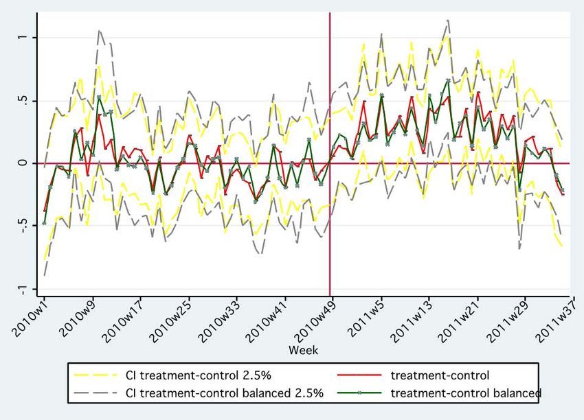
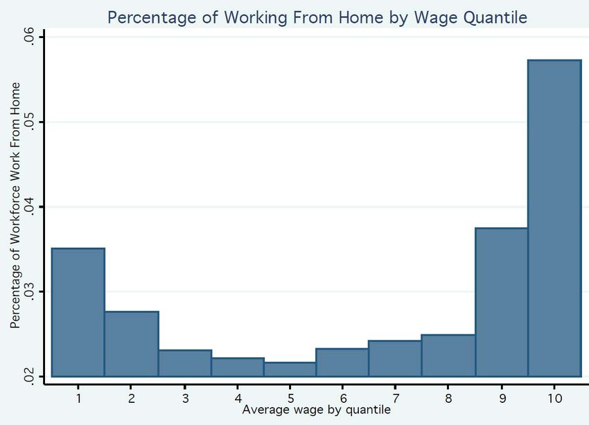
I. INTRODUCTION

Working from home (WFH) is becoming an increasingly common. In the United States over
10% of the workforce reports working from home at least one day a week, while the proportion
primarily WFH has almost doubled from 2.3% in 1980 to 4.3% in 2010 (Figure A1). At the same
time the wage discount (after controlling for observable) from working at home has fallen from
30% in 1980 to zero by 2000 (Oettinger, 2010).

Homeworkers span a wide spectrum of occupations ranging from sales and assistants to
managers and software engineers. Employees that are older, better educated, female and have
children are more likely to work at home. Not surprisingly, working from home is also
significantly more likely in IT intensive industries and occupations. In terms of earnings the
distribution of home-workers is bimodal, with large groups at the bottom and top end of the
wage distribution (Figure A2).

The trade-off between home-life and work-life has also received increasing attention as the
number of households in the US with all parents working has increased from 25% in 1968 to
48% by 2008 (Council of Economic Advisors, 2010). These rising work pressures are leading
governments in the US and Europe to investigate ways to promote work-life balance. For
example, the Council of Economic Advisers (CEA) published a report launched by Michelle and
Barak Obama at the White House in summer 2010 on policies to improve work-life balance. One
of the key conclusions in the executive summary concerned the need for research to identify the
trade-offs in work-life balance policies, stating:

  “A factor hindering a deeper understanding of the benefits and costs of flexibility is a lack
  of data on the prevalence of workplace flexibility and arrangements, and more research is
  needed on the mechanisms through which flexibility influences workers’ job satisfaction
  and firms’ profits to help policy makers and managers alike” (CEA, 2010)

Not surprisingly, given this lack of rigorous empirical evidence, firms are also uncertain about
what policies on home working to adopt. As a result, firms in very similar industries adopt
extremely different practices. For example, in the U.S. airline industry Jet Blue allows all regular
call-center employees to work from home (coming into the office only one day a month), Delta
and Southwest have no home working, and United has a mix of practices. More generally,
Bloom, Kretschmer and Van Reenen (2010) report 39% of US and 37% of European
manufacturing firms offer home working, with a spread of adoption rates in every 3-digit SIC
code surveyed. Thus, the adoption of working from home is an example of a management
practice whose impact is uncertain, and so the adoption is gradual and stochastic, much as in
Griliches’ (1957) classic paper on the adoption of hybrid seed-corn.

Given the uncertainty over the impact of working from home, CTrip – China’s largest travel
agency with 13,000 employees and a $5bn valuation on NASDAQ – wanted to experiment
before deciding whether to implement it across the firm. The motivation was both to reduce
office costs, which were becoming increasingly onerous due to rising rental rates at the Shanghai
headquarter and also to reduce their 50% annual rate of attrition among call center workers. The
executives’ concern was that allowing employees to work at home, away from the supervision of

their shift managers, would have an extremely negative impact on their performance. No Chinese
firm was known to have offered the possibility of working from home to call center employees,
and certainly no controlled experiment with home-work had been publically reported, so this
experiment was unique.

This experiment is also unique because one of the co-authors of this paper (James Liang) is also
the co-founder, first CEO and current Chairman of CTrip. This has provided excellent access not
just to the experimental data, but also to the Ctrip managements’ thinking about the experiment
and its results. The experiment provides detailed insight into the adoption of a new management
practice by a large publicly listed multinational firm, helping to address some of the questions
over the reasons for the non-adoption of other seemingly beneficial management practices.1

In summary, the firm decided to run a nine-month experiment on working from home. They
asked the employees in the Airfare and Hotel divisions whether they would be interested in
working from home four days a week. 2 Approximately half of the employees (508) were
interested. Of these, 255 were qualified to take part in the experiment by virtue of having at least
six months tenure, broadband access and a private room at home (in which they could work).
After a lottery draw, those with even birthdays were selected to work at home while those with
odd birthdates stayed in the office to act as the control group. The home and office employees in
each team had to work the same shift because they worked under a common team manager. The
two groups also used the same IT equipment, faced the same work order flow from a common
central server, and pay system. Hence, the only difference between the two groups was the
location of work. This allows us to isolate the impact of working-from-home (flexi-place) versus
other practices that are commonly bundled alongside this such as different hours (flexi-time).

We found four main results. First, the performance of the home workers went up dramatically,
increasing by 12.2% over the nine month experiment. This improvement came mainly from an
8.9% increase in the number of minutes they worked during their shifts (the time they were
logged in taking calls). This was due to a reduction in breaks and sick-days taken by the home
workers. The remaining 3.3% improvement was because home workers were more productive
per minute worked, apparently due to the quieter working conditions at home. Second, there
were no spillovers on to the rest of the group – interestingly, those remaining in the office had no
change in performance. Third, attrition fell sharply among the home workers, dropping by almost
50% versus the control group. Home workers also reported substantially higher work satisfaction
and attitudinal survey outcomes. Finally, at the end of the experiment the firm was so impressed
by the impact of home-working they decided to roll the option out to the entire firm, allowing the
treatment and control groups to re-choose their working arrangements. Almost one half of the
treatment group changed their minds and returned to the office, while two thirds of the control
group (who initially had requested to work from home) decided to stay in the office. This
highlights how the impact of these types of management practices are also ex ante unclear to
employees.

1
 See, for example, the survey in Bloom and Van Reenen (2011).
2
 Eligible employees were those with 6+ months tenure, a broadband connection at home and access to a quiet room
during their shift. 51% of the employees were eligible according to this criteria (see Table 1).

We are continuing to collect data on current and former employees to evaluate longer-term
impacts on recruitment, promotion and other work and non-work outcomes, and are also
developing an experiment on home-working for managers.
In terms of connections to the wider literature there is an extensive case-study literature on
individual firms which adopt various home working programs. These tend to show large positive
impacts, but are hard to evaluate because of the non-randomized nature of these programs. This
is both true in terms of the selection of firms into working-from home programs, and also the
selection of employees to work at home. For example, as we show in Table 7 when CTrip
allowed a general roll-out of home-working we see high-performing employees choose to move
home and low-performing employees choosing to return to the office, so that the non-
experimental impact of working from home looks substantially two to three times larger than the
experimental impact.
Other related papers include Oettinger’s (2010) piece on the incidence of home-working across
the US, which has been rising rapidly since the 1980s due to increasing use of information-
communication-technologies (ICT), and Bloom, Kretschmer and Van Reenen’s (2010) piece
showing a strong correlation between homeworking practices and productivity and management
practices across firms and countries.
Section II describes the experiment in more detail, while section III presents the results and
section IV provides a set of concluding comments.
II. THE EXPERIMENT
II.A. The Company
Our experiment takes place in Ctrip, a leading travel service provider for hotel accommodation,
airline tickets and packaged tours in China. Ctrip aggregates information on hotels and flights,
and generates revenue through commissions from travel suppliers. The services provided by
Ctrip are comparable to Expedia, Orbitz or Travelocity. Ctrip was established in 1999 and was
quoted on NASDQ in 2003, and is currently worth about $5bn. It is the largest travel agent in
China for number of room in terms of hotel nights and airline tickets booked. The co-founder of
Ctrip, first CEO and the current Chairman is James Liang, who is also currently a Stanford GSB
graduate student and co-author on this paper. This has provided us with unparalleled access to
the company, both in terms of data and experimental design, but also is terms of understanding
the management decision making behind the experiment and roll-out.
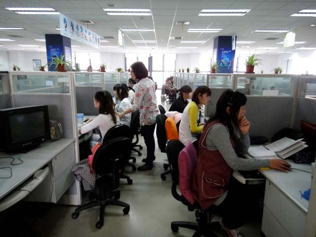
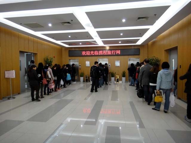
To provide some background on the company Exhibition A displays photos of the Ctrip
headquarters and call center in Shanghai. This is a modern multi-story building that houses the
call center which is running the experiment, as well as several other CTrip divisions and its top
management team. The firm also operates a second larger call center in Nan Tong, outside
Shanghai. Call center employees are organized into small teams of around 10 to 15 people (mean
of 11.7 and median of 11), grouped by department and the type of work. Teams sit together in
one area of the floor, typically occupying an entire aisle. Each team member works in a cubical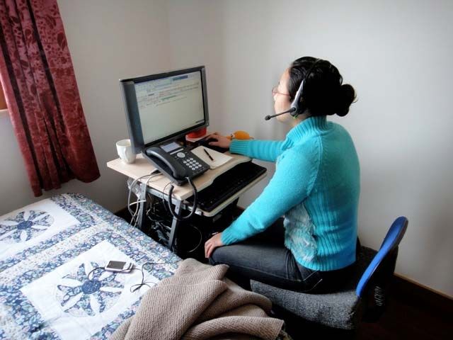
with equipment including a computer, a telephone and a headset. Team leaders patrol the aisles
to monitor employees’ performance as well as helping to resolve issues with reservations.

II.B. The Experimental Design
Ctrip employs about 13,000 employees, of which 7,500 work at two large call centers as
customer service representatives in Shanghai and Nan Tong. Our experiment takes place in the
airfare and hotel booking departments in the Shanghai call center. The representatives’ main job
is to answer phone calls, make reservations, and work to resolve issues on existing bookings.
They typically work 5 shifts a week, scheduled by the firm ahead of time. Employees are
organized by teams, and a team works on the same schedule so individuals do not choose their
shifts. The firm adjusts the length of the shift depending on volume of the bookings.

The treatment in our experiment is to work 4 shifts at home and to work on the 5th shift in the
office on a fixed day of the week. Treatment employees still work on the same schedule as their
teammates because they have to work under the supervision of the team leader (who is always
office based), but operate from home for 4 of their five shifts. For example, in a team the
treatment employees might work from home from 9am to 5pm on Monday, Tuesday, Wednesday
and Friday and from the office from 9am to 5pm on Thursday. The control employees would
work from the office from 9am to 5pm on all five days. Hence, the experiment only changes the
location of work, not the type of work or the hours of work. Since all incoming phone-calls and
work orders are distributed by central servers the work flow is also identical between work and
home locations.

Importantly, individual employees are not allowed to work overtime outside their team shift as
they require their team leader to supervise their work. Hence, entire teams can have their hours
changed – for example all teams had their shifts increased during the week before Chinese New
Year – but no individual is able to work overtime on their own. So the impact of eliminating
commuting time, which is 80 minutes a day for the average employee, on home-workers ability
to work overtime is not a factor directly driving the results.3 Home workers also use the same
CTrip provided computer terminal and phone equipment and software, face the same pay and
promotions structure, and undertake the same training as office workers.

In early November 2010, employees in the airfare and hotel booking departments were informed
of the working from home program. They all took an extensive survey on demographics,
working conditions and their willingness to join the program. Employees who are both willing
and qualified to join the program are recruited for the experiment. To qualify an employee
needed to have tenure of at least 6 months, have broadband Internet at home to connect to the
network, and to have an independent workspace at home during their shift (such as their own
bedroom). 51% of the 996 employees in the airfare and hotel booking departments qualified for
the experiment. Of those 49% were interested in joining the experiment (full details in Table 1).
In the end, 255 employees joined the experiment.

The treatment and control groups were then determined from this group of 255 employees
through a public lottery. Employees with an even birthdate (a day ending 2, 4, 6, 8 etc) were

3
 It could indirectly matter if, for example, employees at home can run household errands in the time saved by not
commuting that employees working from the office have to take breaks to perform.

selected into the treatment and those with an odd birthdate (a day ending 1, 3, 5 etc) were in the
control group. This selection of even birthdates into the treatment group was randomly chosen by
the Chairman, James Liang, by drawing a ping pong ball from an urn in a public ceremony one
week prior to the experiment start date (see Exhibit B).4 Even birthdate employees who had
chosen to be in the experiment group are notified and equipment is installed at each treatment
participant’s home the following week. Odd birthdate employees who had chosen to be in the
experiment acted as the control group. The experiment commenced on December 6, 2010.

The experiment lasted about 9 months. On August 15, 2011, employees were notified that the
experiment had ended and Ctrip would roll out the experiment to those who are qualified and
interested in working at home in the Airfare and Hotels group on September 1st, 2011 (other
groups like Corporate, International and Package have yet to be included in the roll-out).
Throughout the experiment employees were told the experiment would be evaluated to guide
future company policies, but they did not learn the actual policy roll-out until August 15th.
Because of the large scale of the experiment and the lack of dissemination of experimental
results beyond the core management team, employees were uncertain as to the long-run decision
of the firm on roll-out prior to the decision. Employees in the treatment group who wished to
come back to work in the office full-time were allowed to come back on September 1st, but
importantly not before then. Qualified employees in the control group who wished to work at
home were only allowed to do so after the practice was rolled out to the whole firm on August
15th, and could then request to have the equipment installed in their home.

Figure 1 shows compliance with the experiment throughout the experimental period until the end
of December 2011. The percentage of treatment group working at home shot up to 90% within
two weeks of the commencement of the experiment. It hovered between 80% and 90%
throughout the experimental period and dropped sharply after the experiment ended in late
August. Then it stabilized at around 60% through the rest of the year. The compliance does not
reach 100% during the experiment mainly due to technical reasons - mainly that the Broadband
speed was not fast enough or the employee moved apartment and lost access to their own room.5
The control group worked in the office full-time during the experiment.

Since compliance was not perfect our estimators take even birthdate status as the treatment
status, so we estimate an intention to treat result. Given we are interested in evaluating the
impact of a policy of allowing home-working this seemed appropriate.

II.C. The Experimental Motivation
Ctrip was interested in running the experiment to investigate the impact of allowing employees
to work from home. They believed allowing employees to work from home would allow them to
save on office space, cut down turnover, and reduce labor costs by tapping into a wider pool of
workers, such as people living too far outside Shanghai to commute in on a daily basis but close
4
  It was important to have this draw in an open ceremony so that managers and employees could not complain of
“favoritism” in the randomization process. The choice of odd/even birthdate was made deliberately to make the
randomization process straightforward and transparent.
5
  In all estimations we use the even birthdate as the indicator for working-at-home so these individuals are treated as
home workers. In a probit for actually working from home during the experimental period none of the observables
are significant suggesting (see Appendix Z) so it appears this returning to the office was pretty random. One reason
is that IT group policed this to prevent employees fabricating stories to enable them to return to the office.
enough to commute in on a weekly basis. But they were uncertain on the impact of allowing
employees to work from home on their performance. Their workforce is primarily younger
employees, many of which may struggle to remain focused working from home.

Since no other Chinese firm had moved to allowing home-working amongst its call center
employees there was no local precedent. In the US the decision to allow employees in call
centers to work from home varies across firms, even those within the same industry, suggesting a
lack of any consensus on its impact. For example, in the airline industry while Jet Blue and
American Airlines allow home-working, British Airways, Continental, Delta and Southwestern
do not, and United is experimenting with a mixed model. The prior academic literature on call
centers also offered limited guidance, being based on case-studies of individual firm-level
interventions.

II.D. Data Collection
Ctrip has an extremely comprehensive central data collection system. One of its founders,
including James Liang, came from Oracle so had extensive database software experience. The
majority of data we use in our paper are directly extracted by from the firms’ central database,
providing extremely high data accuracy. The data we collected can be categorized in 5 fields:
performance, labor supply, attrition, reported employee work satisfaction, detailed demographic
information and surveys on attitudes towards the program.

Performance measures vary by the type of workers, as detailed in Appendix 1. In summary, we
have 4 types of workers and 6 different performance measures in our sample. We have 137 order
takers, 71 order placers, 36 order correctors, and 11 night shift workers. Order takers main tasks
are to answer phone calls and record orders in the Ctrip system. Their key performance measures
are the number of phone calls answered and number of orders taken. Order placers process the
orders by contacting the hotels and notify clients of confirmed reservations. Their key measures
are numbers of different types of confirmation phone calls and notification phone calls
depending on the department. Order correctors resolve issues on existing reservations such as
overbooking, etc. Their key measure is the number of orders corrected. Night shift workers cover
responsibilities of both order placers and order correctors at night, typically from 11PM to 7AM.

For order takers, minutes on the phone is a direct and accurate measure of time spent working.
We have logs of phone calls and call lengths from the central database of Ctrip. The firm also
uses this measure to monitor work of their employees. We also calculate phone calls answered
by minute on the phone as a measure of labor productivity for this type of workers.

We have daily key performance measures of all employees in the airfare and hotel booking
departments from January 1st, 2010 to December 25th, 2011. We also have daily minutes on the
phone for order takers during the same period. We have detailed daily records of hours of leave
from the airfare department by types of leave from September 1st, 2010 to August 15th, 2011.
We know the date and reason of employees in the experiment quitting the experiment or leaving
the firm. We have data from weekly survey of the employees in the experiment on work
exhaustion, positive and negative attitudes (See details in Appendix A2). Lastly, we designed
and conducted two rounds of surveys in November 2010 and August 2011. From the surveys and
the company database, we collect detailed information on all the employees in the two
departments including basic demographics, income, attitudes toward the Program.

                                        III. RESULTS

III.A. Performance Regressions
We start by estimating the intention to treat equation

OUTCOMEi,t = aTREATi × EXPERIMENTt + bt + ci +ei,t                                        (1)

We start by estimating the impact of work-from-home (WFH) Program via equation (1).
TREAT is a dummy variable that equals 1 if an individual belongs to the treatment group defined
by having an even-numbered birthday. EXPERIMENT is a dummy variable that equals 1 for
weeks after the experiment started on December 6th. OUTCOME is one of the key measures of
work performance including an overall performance z-score measure, log of weekly phone calls
answered, log of phone calls answered per minute on the phone, and log of weekly sum of
minutes on the phone. bt incudes a series of week dummies to account for seasonal variation in
traveling demand such as the World Expo in 2010 and the Chinese New Year. ci is the individual
fixed effect that includes non-time-varying individual idiosyncratic factors that affect work
performance.

Overall performance z-score is a measure to make performance of different types of workers
comparable. First we generate weekly sum of key measures of performance for each type of
workers. For example, order takers have two key measures of performance—phone calls
answered and orders placed. To obtain z scores of each key measure, we subtract the weekly sum
by pre-experiment mean by department of the key measure, and divide it by pre-experiment
standard deviation. Then we average the key measure z-scores within each type to generate an
overall performance z-score measure. Finally, we normalize this measure again by subtract the
pre-experiment mean and divide by the pre-experiment standard deviation to create the final
double z-scored overall performance measure. This measure has mean 0 and standard deviation 1
over the pre-experiment period.

In column (1) of Table 2, overall performance of the treatment group is 0.2 standard deviations
higher than the control group after the experiment started. The result is very significant at 1%.
We can also see the results from Figure 2 where overall performance of the treatment group and
the control group are plotted from Jan 1st 2010 to August 15th 2011. The red vertical line is when
the experiment started. The black solid line represents the treatment group and the red solid line
represents the control group. Before the experiment started, despite seasonal variations, the
treatment group trends closely with the control group. After 6 weeks of the experiment, treatment
group starts to differ from the control group, and the difference is quite consistent until the last
few weeks of the experiment.
The largest type of workers we have in our sample are the 137 order takers. If we limit the
sample to the order takers, we can use phone calls answered as the key performance measure for
all the order takers. The z-scores of phone calls account for different volume and average length
of phone calls in two departments. Column (2) shows that order takers in the treatment group
answer 0.249 standard deviation more phone calls than the control group after the experiment
started. We also use log of weekly phone calls as the outcome variable. We see that the treatment
group answers 11.7% more phone calls than the control group, as shown in column (3).

We further decompose the difference in performance observed in column (3) into phone calls
answered per minute on the phone, a measure of productivity, and minutes on the phone, a
measure of labor supply. Column (4) and (5) suggest that out of the 11.7% difference in
performance between the treatment group and the control group, 3.4% is accounted for by
difference in productivity, and 8.4% is accounted for by difference in labor supply. One question
is that whether quality of the service has been compromised as a tradeoff for the increase in
productivity in the treatment group. We construct two quality measures: conversion rate and
weekly recording scores. Conversion rate is calculated as the percentage of phone calls answered
resulting in orders. The first two columns of Appendix A3 show that the treatment group does
not differ in conversion rate from the control group during the experiment. Phone calls are all
recorded and sampled for quality control by the company on a weekly basis. The last two
columns of Appendix A3 show that treatment group maintains the same level of recording scores
as the control group.

From visual examination of Figure 2, the impact of the experiment appears to have varied over
time. Specifically, during the first 6 months of the experimental period, treatment group seems to
perform better than the control group, but the difference appears to be smaller during the last 3
months of the experimental period. We formally test this by interacting number of weeks since
the experiment started with experiment and treatment. Appendix A7 shows that there is no linear
weekly trend in performance gap between treatment and control group.

III.B. Labor Supply Regressions
In Table 3, we investigate further factors that contribute to difference in labor supply. Order
takers may adjust labor supply in three different ways. First, they may spend more minutes
answering the phone for each hour of their shift. Second, they may take fewer hours off for each
shift. Third, they may take fewer shifts off.

Because we have accurate records of hours of leave from the airfare booking department only,
we limit the sample further to 89 order takers in the airfare department. Column (2) of Table 3
shows that these order takers are not different from those in the hotel booking department in
labor supply (results are very similar to the full group in Column (1)). Column (3)-(5) suggest
that out of 8.95% difference in labor supply between the treatment and the control group 6.7% is
accounted for by taking fewer hours off each shift and 3.9% is accounted for by taking fewer
shifts off.

Again we divide the sample period into first 6 months and last 3 months to investigate what
contributes to the reduction in the minutes worked gap between treatment and control group
during the last 3 months of the experiment. Looking at the bottom panel of Table 3 we find it is
because the gap in hours per day worked equalizes between the treatment and control group over
this period, because working the office relative to home becomes substantially more attractive
due to the comfort value of having air-conditioning.6

III.C. Spillovers and comparisons with two “quasi” control groups
Is the gap between treatment and control caused by the treatment group performing better or the
control group performing worse? In Table 4, we collect data on two other “quasi” control groups
to answer this question. The first group is the eligible employees in the Nan Tong call center.
This is CTrip’s other large call center, located in Nan Tong, a city about 1 hour drive outside of
Shanghai. This call center also has airfare and hotel departments, and calls are allocated across
the Shanghai and Nan-Tong call centers randomly. The second group is the 253 eligible
employees that did not volunteer to participate in the WFH experiment in the Shanghai call
center. These are the individuals that were eligible for the experiment (own room, 6+ months of
tenure and broadband) but did want to work from home (those in Table 1 column (2) but not in
column (3)). We think these two groups are comparable to the treatment and control groups for
two reasons. First, all four groups face the same demand for their service. Second, they all meet
the requirements for eligibility to participate in the experiment.

Figure 3 shows that the performance of the eligible group in the Nan Tong call center tracks that
of the treatment and control well before the experiment. After the experiment started, the
performance of the Nan Tong group is similar to that of the control group. Results in the top
panel of Table 4 confirm this finding. Differences in overall performance, efficiency and labor
supply between the control group and the Nan Tong eligible group is statistically insignificant
from zero. The bottom panel compares treatment and control group to the eligible non-
experimental group in Shanghai. Again we find no difference between the control group and the
eligible non-experimental group. These results suggest that the gap between the treatment and
control group mainly reflects an improvement in performance, efficiency and labor supply of the
treatment group rather than any deterioration of the control group. That is, although the control
group and the treatment group work in the same team we find little evidence of the control group
being discouraged by not able to work at home.

We also look for spillovers by examining the variation in the number of individuals randomly
assigned to treatment across the groups within the Shanghai office. Because groups are small,
random variations in the number of employees with even and odd birthdays generates variations
in the number of employees that get to work at home. We use this (the share of even in the
eligible volunteered group) to instrument for the share of all employees working from home, and
investigate the impact of this on the team’s performance. As we show in Table A4 we again find
no evidence for spillovers across individuals from home-working.

III.D. Attrition
One of the reasons Ctrip is interested in running the experiment is to retain workers. Turnover
rate in Ctrip call center representatives has been historically hovered around 50% per year, which
is typical of the call center industry in China. Management estimates that hiring and training a
representative costs on average $2000, about 6 months salary of an average employee. Figure 4

6
 The control group tend to arrive earlier and leave later from work because it is much cooler, while the treatment
group apparently work fewer minutes at home because of the heat.
plots the cumulative attrition rate of treatment and control group separately over the
experimental period. Shortly after the commencement of the experiment, cumulative attrition
rates diverged between the two groups and the difference is statistically significant. By the end of
the experiment, attrition rate in the treatment group (17%) is nearly half as that in the control
group (35%).

We further test whether selective attrition exists by running probit regressions. The dependent
variable is whether an employee quits the job during the experimental period between December
6th 2010 and August 15th 2011. Column (1) in Table 5 confirms the finding in Figure 4. Column
(2) and (3) test whether employees with worse performance before the experiment are more
likely to attrite in treatment group compared to control group. Pre-experiment performance is the
average of individual weekly performance z-scores during the pre-experimental period from
January 1st 2010 to December 5th 2010. We find no evidence that such is the case. We find that
younger employees and those with higher cost of commute are more likely to quit their job.

In column (4) and (5), we use the same specifications as in column (2) and (3) but replace the
pre-experiment performance with post-experiment performance. Post-experiment performance is
the average of individual weekly performance z-scores during the post-experimental period from
December 6th 2010 to August 15th 2011. We find that in both groups employees with worse
performance during the experiment are more likely to attrite, but they are more likely to attrite in
control group compared to treatment group. The difference is statistically significant, but the
impact of the performance gap between the treatment and control groups is quantitatively
negligible as Appendix Figure 1 shows.

Given these attrition results we also investigated if different characteristics were related to
differential performance changes from working at home. Appendix A5 interacts a series of
different characteristics of the employees – such as marital status, children and commute time –
with the treatment*experiment term but finds no significant relationship. One of those
characteristics is pre-experiment performance. Again we find no differential treatment effect by
the pre-experiment performance level.7 This suggests while different types of employees have
different tendencies to volunteer to work from home and stay in the job (rather than quit) the
impact of working from home on their performance is similar across these groups.

III.E. Employee Self-reported outcomes
Ctrip management is also interested to find out how employee self-reported well-beings are
impacted by the Program. They ran two sets of surveys: the satisfaction survey and emotion
survey. Details of survey questions and methodology are listed in Appendix A2, but in summary
these are reasonably standard employee satisfaction tests developed by Christina Maslach and
Susan Jackson in the 1970s (see for example Maslach and Jackson, 1981). The satisfaction
survey was conducted five times throughout the experimental period. Once in early November
before the randomization took place and four times after the experiment had started. Since the
employees were unaware of the assignment at the initial survey, the first survey is a credible
baseline. The first three columns of Table 6 show three different satisfaction measures. The

7
 We also create dummy for pre-experiment performance quintiles and interact them with treatment*experiment. For
example, we interact bottom 25 percent with treatment*experiment, and we do not find the bottom 25 percent of the
workers have different treatment effect from the rest of the workers.
treatment group reports no different satisfaction level from the control group at the first survey,
but the treatment group reports statistically significantly higher satisfaction level throughout the
experiment.

The emotion survey is conducted every week. The first week was conducted in late-November
2010, before the experiment began but after the randomization so that individuals had been
informed of their status in the treatment or control groups. Although not consistently statistically
significant, the treatment group already reports higher positive attitude, less negative attitude and
less exhaustion from work upon learning their assignment but before changing their location of
work. After starting the experiment the gap between the treatment and control group rose further,
so that treatment group reported statistically significantly higher positive attitude and less work
exhaustion.

III.F. Employees’ views toward the Program
We designed a survey to inquire employees’ views toward the Program as well as collecting
demographic information. We administered the same survey with the help of the Ctrip
management in November 2010 and August 2011. Employees are asked specifically whether
they are interested in participating in the Work-at-Home Program if they were eligible. They can
choose from three answers: yes, no or undecided. For the November 2010 survey employees
were not told the eligibility rules in advance of the survey (i.e.: own room, 6+ months tenure,
internet connect etc). For the November 2011 survey they were told the experiment was being
rolled out to the company, but again not what the criteria for this would be.

In Table 7 Panel A, we tabulate employees answers in November 2010 against August 2011. The
sample includes 568 employees who answered both surveys. In November 2010, 51% of the
employees are willing to work at home, compared to 40% in August 2011. More then 53% of the
employees maintained their positions in both surveys, evidenced by the weights on the diagonals.
About 20% of those who answers yes in the first survey decided they were not interested in the
second survey where 12% of those who initially were not interested showed interest in the
second survey.

III.G. Roll-out and Switch
In August 2011 the management took the decision to roll-out the experiment to the entire firm.
The experiment was evaluated to be a clear success, with the estimated savings per employee
working-from-home estimated to be at least $2,000 (see Appendix Figure A3). On August 15th,
2011, employees were notified that the experiment had ended and Ctrip would roll out the
experiment to those who are qualified and interested in working at home on September 1st.
Employees in the treatment group who wished to come back to work in the office full-time were
allowed to come back at the beginning of September. To understand the characteristics of the
workers who choose to come back to the office, we run probit regressions using whether a
worker returns to the office as the outcome. The sample for returning to the office includes the
103 treatment works still at CTrip at the end of the experiment. Out of the 103 treatment
workers, 22 opt to come back to work in the office full-time. As shown in column (3) of Table 7
Panel B, we find that employees who have better pre-experiment performance and worse post-
experiment performance are more likely to return to the office. They are likely a group of
employees who did not benefit as much from the Work-from-Home Program. We also find that
married employees or those living with parents are less likely to return to the office. In-depth
interviews with the employees as well as home visits suggest that these employees tend to
benefit more from the Program as they enjoy spending more time with their family and have
received support from their family as well.

Other qualified employees who wish to work at home gradually went home after equipment was
installed at the beginning of November. The sample for moving home includes the 73 employees
from the control group who still remain by the end of the experiment. 27 out of the 73 employees
choose to work at home. We do not find correlation between performance and switch to work at
home, but we do find that older employees are more likely to work at home.

                                    IV. CONCLUSIONS

The frequency of working from home has been rising rapidly in the US, with over 10% of the
work-force now reporting regular home working. But there is uncertainty and skepticism over
the effectiveness of this, highlighted by phrases like “shirking from home”. We report the results
of the first randomized experiment on home-working, run in a 13,000 employee NASDAQ listed
Chinese firm. Employees that volunteered to work from home were randomized into 9-months of
home-working by even/odd birth-date. We find a highly significant 12% increase in performance
from home-working, of which 8% is from working more minutes of their shift period (fewer
breaks and sick-days) and 3% from higher performance per minute. We find no negative
spillovers onto workers left in the office. Home workers also reported substantially higher work
satisfaction and psychological attitude scores, and their job attrition rates fell by over 50%.
Interestingly, the impact of home-working was ex ante unclear both to the firm and the
employees. The firm ran to experiment to evaluate its impact, and after the experiment was so
enthusiastic it decided to permanently roll out the practice. The employees’ response was much
more heterogeneous, with about one third of employees switching practices after the end of the
experiment. This highlights how the impact of management practices like home-working is
unclear to firms and employees, helping to explain their slow adoption over time.
V. BIBLIOGRAPY (to be completed) Bloom, Nick and Van Reenen, John, (2011), “Human resources and management practices”, Handbook of Labor Economics, Volume 4, edited by Orley Ashenfelter and David Card. Bloom, Nick, Tobias Kretschmer and John Van Reenen, (2009), “Work-life Balance, Management Practices and Productivity’, in International Differences in the Business Practice and Productivity of Firms, Richard Freeman and Kathy Shaw (eds). Chicago: University of Chicago Press. Council of Economic Advisors (2010), “Work-life balance and the economics of workplace flexibility”, http://www.whitehouse.gov/files/documents/100331-cea-economics-workplace- flexibility.pdf Griliches, Zvi (1957), “Hybrid Corn: An Exploration in the Economics of Technological Change”, Econometrica, volume 25 (4), pp. 501-522. Maslach, C., & Jackson, S.E. (1981). Maslach Burnout Inventory. Research edition. Palo Alto, CA: Consulting Psychologist Press. Oettinger, Gerald (2012), “The Incidence and Wage Consequences of Home-Based Work in the United States, 1980-2000”, Journal of Human Resources forthcoming
DATA APPENDIX
Appendix A1: Table for different types of workers and their key performance measures

                                                                                   Number of
 Types of Workers            Department       Key Performance Measures
                                                                                 Workers
                                Airfare       Phone Calls Answered                     89
 Order Takers
                                Hotel         Orders Taken                             48
                                Airfare       Notifications Sent                       46
 Order Placers
                                Hotel         Reservation Phone Calls Made             25
 Order Correctors               Hotel         Orders Corrected                         36
                                              Reservation Phone Calls Made
 Night Shift Workers            Hotel                                                    11
                                              Orders Corrected

Appendix A2: Explanations on the Work Satisfaction Survey

Work Exhaustion: CTrip’s in-house psychology counselors use an adapted excerpt from the
Maslach Burnout Inventory Survey to measure the emotional exhaustion of the employees from
work. The MBI survey was developed by Berkeley psychologist Christina Maslach and Susan
Jackson in the 1970s (see Maslach and Jackson, 1981).

Each employee is asked to evaluate his or her “emotional exhaustion” at the end of the work
week. The survey contains 6 questions. Each employee is asked to report how often he has felt
the way described at work during the week: feel this way every day, almost all the time, most of
the time, half of the time, a few times, rarely, never. The survey questions are listed below:
    1. I feel emotionally drained from my work.
    2. I feel used up at the end of the work day.
    3. I dread getting up in the morning and having to face another day on the job.
    4. I feel burned out from my work.
    5. I feel frustrated by my job.
    6. I feel I am working too hard on my job.

Positive and Negative Attitudes: CTrip’s in-house psychology counselors use an adapted 16-item
Positive and Negative Affect Schedule (PANAS) developed by Clark and Tellegen in 1988 to
measure the positive and negative attitudes of the employees.

The survey comprises two mood scales, one measuring positive affect and the other measuring
negative affect. Each item is rated on a 5-point scale ranging from 1 = very slightly or not at all
to 5 = extremely to indicate the extent to which the employee feels this way the day he takes the
survey. To evaluate the positive affect, psychologists sum the odd items. In cases with internally
missing data (items not answered), the sums were computed after imputation of the missing
values: # items on scale / # actually answered, multiplied by the sum obtained from the answered
items. A higher score indicates more positive affect, or the extent to which the individual feels
enthusiastic, active, and alert. The negative affect is evaluated similarly by summing up the even
items.
The 16 items are listed below. 1. Cheerful 2. Jittery 3. Happy 4. Ashamed 5. Excited 6. Nervous 7. Enthusiastic 8. Hostile 9. Content 10. Guilty 11. Relaxed 12. Angry 13. Proud 14. Dejected 15. Active 16. Sad
Appendix A3: Quality did not change in the experiment

                                     (1)                  (2)                    (3)                      (4)
 Dependent Variable           recording grade       recording grade     conversion (z score)     conversion (z score)
 Individual FE                       No                   Yes                   No                       Yes
 Week fixed-effects                 Yes                   Yes                   Yes                      Yes
 Experiment*Treatment              -0.007                -0.006                -0.026                   -0.026
                                   (0.008)              (0.008)               (0.071)                  (0.065)
 Treatment                         0.000                                       -0.011
                                   (0.005)                                    (0.091)
 Number of Employees                 89                    89                   135                      135
 Number of Weeks                     87                    87                    87                       87
  Observations                      5689                   5689                 9815                     9815
Notes: Sample in the first two columns includes 89 order takes in the airfare department (for which we can obtain
recording grade information). The sample in the last two columns includes 135 order takers in airfare and hotels (the
group for which conversion rate data exists). Clustered standard errors. *** denotes 1% significance, ** 5%
significance and * 10% significance.
Appendix A4. Lack of any obvious cross-sectional Spillover effects
(1) (2) (3) (4)
Dependent variable Overall Performance Overall Performance Overall Performance Overall Performance
Sample Non-experiment Control Treatment Non-experiment + Control
Specification IV IV IV IV
Treat/Total -0.221 -0.574 -0.523 -0.263
(0.398) (0.392) (1.039) (0.357)
Week FE Yes Yes Yes Yes
No. of Teams 79 59 56 79
Observations 36660 8218 9587 44846
R-squared 0.410 0.359 0.467 0.398
IV first stage IV first stage IV first stage IV first stage
Sample Non-experiment Control Treatment Non-experiment + Control
Dependent variable Treat/Total Treat/Total Treat/Total Treat/Total
Treat/(Treat+Control) 0.253*** 0.390*** 0.219*** 0.264***
(0.0226) (0.0295) (0.0484) (0.0236)
Week FE Yes Yes Yes Yes
No. of Teams 79 59 56 79
Observations 36660 8218 9587 44846
R-squared 0.881 0.903 0.891 0.874
Notes: “Treat/total” is the number of employees in treatment divided by the number of employees in each team. A team is composed
of 10 to 20 employees who specialize in the same type of tasks and work the same schedule of shifts. Each team is monitored by the
same team leader. “Treat/(Treat+Control)” is the number of employees in treatment divided by the number of employees in treatment
and control group within each team. Both “Treat/total” and “Treat/(Treat+Control)” are set to zero before the experiment started on
December 6, 2010. “Treat/(Treat+Control)” is fixed at the beginning of the experiment. “Non-experiment”, “Control” and
“Treatment” refer to employees from each group. The sample includes data from January 1, 2010 to August 15, 2011. Clustered
standard errors. *** denotes 1% significance, ** 5% significance and * 10% significance.Appendix A5. Panel A: Treatment Effects Seem Homogeneous across Characteristics
Performance (1) (2) (3) (4) (5) (6) (7) (8) (9) (10) (12)
Commute short prior short live w/ live w/ live w/ pre-exper
Child Female renter young
>120min experience tenure parents spouse friends performance
experiment x 0.0788 -0.106 0.155 -0.111 -0.0430 0.0559 -0.0544 0.0127 -0.0132 -0.126 0.0963
treat x (0.184) (0.130) (0.146) (0.148) (0.132) (0.134) (0.135) (0.141) (0.178) (0.253) (0.104)
"characteristic"
experiment x -0.0395 0.105 -0.0612 0.0764 0.00864 0.0493 0.0730 0.0171 -0.0244 0.213 -0.312***
"characteristic" (0.133) (0.0919) (0.0955) (0.109) (0.0946) (0.0973) (0.0971) (0.105) (0.120) (0.210) (0.0812)
experiment x 0.216*** 0.278*** 0.171** 0.243*** 0.249** 0.208** 0.257** 0.208* 0.217*** 0.223*** 0.221***
treatment (0.0711) (0.101) (0.0831) (0.0781) (0.106) (0.0974) (0.112) (0.120) (0.0688) (0.0692) (0.0616)
Observations 17611 17611 17603 17526 17611 17611 17611 17526 17526 17526 17611
R-squared 0.417 0.417 0.416 0.416 0.417 0.417 0.417 0.416 0.416 0.417 0.423
Notes: The performance z-scores are constructed by taking the average of normalized performance measures (normalizing each
individual measure to a mean of zero and standard deviation of 1 across the sample). The sample includes data from January 1, 2010
to August 15, 2011. “young” equal 1 if an employee is under 24. “Short prior experience” equals 1 if an employee with less than 6
months of experience before joining Ctrip. “Short tenure” equals 1 if an employee has worked in Ctrip for less than 24 month by
December 2010. “Pre-exper performance” is the average z-score of performance between Jan 1, 2010 and Oct 1, 2010 for each
employee. Clustered standard errors. *** denotes 1% significance, ** 5% significance and * 10% significance.Appendix A6: The top 15 occupations for numbers working Profession Number Working At Home % Working At Home Sales 697,879 8.6% Managers 658,577 11.8% Childcare and homecare aides 327,851 13.1% Accountants and auditors 215,959 5.1% Data analysts 146,983 22.5% Software developers and programmers 129,860 8.2% Designers and artists 124,563 8.0% Secretaries and assistants 120,260 3.4% Chief executives and legislators 94,807 9.2% Writers and authors 70,493 38.5% Customer service representatives 64,983 3.0% Military tactical specialists 62,977 31.6% Lawyers and judges 55,594 5.5% Post-secondary teachers 48,401 3.7% Carpenters 43,317 3.8% All Notes: The numbers are from authors’ calculation based on 2010 Census IPUMS 1% sample.
Appendix A7: The performance impact of working from home by week
                                                (1)                      (2)                    (3)                       (4)                         (5)
 Dependent Variable                   Overall Performance            Phonecalls             Phonecalls          Phonecalls Per Minute       Minutes on the Phone
 Dependent Normalization                     z-score                  z-score                   log                      log                          log

 Period: 11 months pre-experiment and 9 months of experiment
 Experiment*Treatment*Week                    -0.001                   -0.003                 -0.001                    -0.000                      -0.002
                                             (0.004)                  (0.004)                 (0.002)                  (0.000)                      (0.002)
 Experiment*Treatment                        0.216**                 0.303***                0.140***                  0.034**                     0.121***
                                             (0.100)                  (0.087)                 (0.041)                  (0.015)                      (0.046)

 Number of Employees                           255                      137                     137                      137                          137
 Number of Weeks                                87                       87                     87                        87                          87
 Observations                                 18125                     9817                   9817                      9817                        9817
Notes: The regressions are run at the individual by week level, with a full set of individual and week fixed effects. Experiment*treatment is the interaction of the
period of the experimentation (December 6th 2010 until August 15th 2011) by an individual having an even birthdate (2nd, 4th, 6th, 8th etc day of the month).
Experiment*treatment*week is the interaction of this with the number of weeks the experiment has been running. The pre period refers to January 1st 2010 until
December 5th 2010. Week is calculated as the number of weeks since started. Week equals zero prior to December 6th, 2010. The z-scores are constructed by
taking the average of normalized performance measures (normalizing each individual measure to a mean of zero and standard deviation of 1 across the sample).
Since all employees have z-scores but not all employees have phonecall counts (because for example they do order booking) the z-scores covers a wider group of
employees. Minutes on the phone is recorded from the call logs. Standard errors are clustered at the individual level. *** denotes 1% significance, ** 5%
significance and * 10% significance.
Appendix Figure A1: Proportion of the workforce working mainly at home has grown steadily from 2.3% in 1980 to 4.3% in 2010.
Appendix Figure A2: Home workers are bi-modally distributed
across the earnings spread
Appendix Figure A3: Using a balanced panel, we observe the
same performance gap between treatment and control group.
Appendix Figure A4: Impact of the Program on Firm Profitability

•   Office space: Imputed rent for Shanghai HQ is $5m per year. 1/4 of
    space is taken up central management and the rest by 3000 call
    center employees. Hence, estimated office space saving per
    employee is $1,250 per year

•   Wages: Performance of the treatment group rises by about 7.5%.
    Salaries are about 50% performance based and 50% fixed. Given
    average salaries of about $10,000 per year implies a saving per
    employee of about $375

•   Retention: CTrip estimates hiring and training cost per employee of
    $2000, so that reducing attrition from 40% to 20% p.a. reduces
    retention costs by about $400 per year.

Ignores: hiring and wage impact (probably positive), long-term
performance impact (ambiguous), and assumes quality and capital
equipment requirements are unchanged (as they were in the experiment)
Table 1. Summary Statistics
Variable Total Volunteered t-stat Experiment t-stat
(to work (volunteered (volunteered, (experiment v
from home) v total) own room, 6+ total)
months tenure)
Number of people 996 508 251
Age 23.2 23.2 0.032 24.4 7.232
Male 0.32 0.34 1.192 0.46 5.607
Married 0.15 0.18 2.202 0.27 6.348
Education (omitted group is high school)
tertiary technical school 0.39 0.35 -2.461 0.34 -1.690
University 0.02 0.02 -0.095 0.02 -0.270
Prior work experience (months) 10.8 12.8 3.172 17.9 6.691
Tenure (months) 24.9 23.1 -2.733 26.8 1.607
Children (1=yes) 0.09 0.11 2.291 0.18 5.896
Rental 0.50 0.49 -0.574 0.22 -11.01
Age of youngest child (years) 0.26 0.36 2.578 0.61 5.470
Live with child 0.06 0.07 1.411 0.12 4.380
Grandparents provide childcare 0.07 0.09 1.998 0.15 5.170
Commute (minute/daily) 80.6 86.5 3.389 112.2 10.82
Cost of commute (yuan/daily) 5.54 6.30 3.431 8.33 7.279
Internet 0.99 1.00 2.193 1.00 0.99
Independent bedroom 0.60 0.66 3.909 1.00 16.23
compensation (yuan/month)
Basewage 1541 1529 -2.501 1536 -0.608
Bonus 990 950 -1.821 1015 0.676
Overtime 119 115 -1.826 124 1.337
Benefit 222 234 1.983 265 4.152
Notes: The total sample covers all CTrip employees in their Shanghai Airfare and Hotel group. Willingness to
participate is based on the initial survey in Nov 2010. Employees were not told the eligibility rules in advance of the
survey (i.e.: own room, 6+ months tenure, internet connect etc). Compensation is calculated as a monthly average of
salary from Jan 2010 to Sep 2010 (note that 1 Yuan is about 0.15 Dollars). The t-stat in the second column tests
whether differences between volunteered employees and all employees are significant, while those in the last
column tests whether differences within the volunteered group between eligible and all employees are significant.Table 2: The performance impact of working from home
(1) (2) (3) (4) (5)
Dependent Variable Overall Performance Phonecalls Phonecalls Phonecalls Per Minute Minutes on the Phone
Dependent Normalization z-score z-score log log log
Period: 11 months pre-experiment and 9 months of experiment
Experiment*Treatment 0.226*** 0.263*** 0.122*** 0.033** 0.089***
(0.064) (0.064) (0.026) (0.013) (0.028)
Number of Employees 255 137 137 137 137
Number of Weeks 85 85 85 85 85
Observations 17778 9503 9503 9503 9503
Notes: The regressions are run at the individual by week level, with a full set of individual and week fixed effects. Experiment*treatment is the interaction of the
period of the experimentation (December 6th 2010 until August 20th 2011) by an individual having an even birthdate (2nd, 4th, 6th, 8th etc day of the month). The
pre period refers to January 1st 2010 until December 5th 2010. The z-scores are constructed by taking the average of normalized performance measures
(normalizing each individual measure to a mean of zero and standard deviation of 1 across the sample). Since all employees have z-scores but not all employees
have phonecall counts (because for example they do order booking) the z-scores covers a wider group of employees. Minutes on the phone is recorded from the
call logs. Standard errors are clustered at the individual level. *** denotes 1% significance, ** 5% significance and * 10% significance.You can also read