Drug-Target Interaction Prediction via an Ensemble of Weighted Nearest Neighbors with Interaction Recovery
←
→
Page content transcription
If your browser does not render page correctly, please read the page content below

Noname manuscript No.
                                        (will be inserted by the editor)

                                        Drug-Target Interaction Prediction via an Ensemble
                                        of Weighted Nearest Neighbors with Interaction
                                        Recovery

                                        Bin Liu · Konstantinos Pliakos ·
                                        Celine Vens · Grigorios Tsoumakas

                                        Received: date / Accepted: date
arXiv:2012.12325v3 [cs.LG] 9 Jul 2021

                                        Abstract Predicting drug-target interactions (DTI) via reliable computa-
                                        tional methods is an effective and efficient way to mitigate the enormous costs
                                        and time of the drug discovery process. Structure-based drug similarities and
                                        sequence-based target protein similarities are the commonly used information
                                        for DTI prediction. Among numerous computational methods, neighborhood-
                                        based chemogenomic approaches that leverage drug and target similarities to
                                        perform predictions directly are simple but promising ones. However, existing
                                        similarity-based methods need to be re-trained to predict interactions for any
                                        new drugs or targets and cannot directly perform predictions for both new
                                        drugs, new targets, and new drug-target pairs. Furthermore, a large amount
                                        of missing (undetected) interactions in current DTI datasets hinders most DTI
                                        prediction methods. To address these issues, we propose a new method denoted
                                        as Weighted k-Nearest Neighbor with Interaction Recovery (WkNNIR). Not
                                        only can WkNNIR estimate interactions of any new drugs and/or new targets
                                        without any need of re-training, but it can also recover missing interactions
                                        (false negatives). In addition, WkNNIR exploits local imbalance to promote
                                        the influence of more reliable similarities on the interaction recovery and pre-

                                        Bin Liu (Corresponding Author)
                                        School of Informatics, Aristotle University of Thessaloniki, Thessaloniki 54124, Greece
                                        E-mail: binliu@csd.auth.gr
                                        Konstantinos Pliakos
                                        KU Leuven, Campus KULAK, Dept. of Public Health and Primary Care, Kortrijk, Belgium
                                        ITEC, imec research group at KU Leuven
                                        E-mail: konstantinos.pliakos@kuleuven.be
                                        Celine Vens
                                        KU Leuven, Campus KULAK, Dept. of Public Health and Primary Care, Kortrijk, Belgium
                                        ITEC, imec research group at KU Leuven
                                        E-mail: celine.vens@kuleuven.be
                                        Grigorios Tsoumakas
                                        School of Informatics, Aristotle University of Thessaloniki, Thessaloniki 54124, Greece
                                        E-mail: greg@csd.auth.gr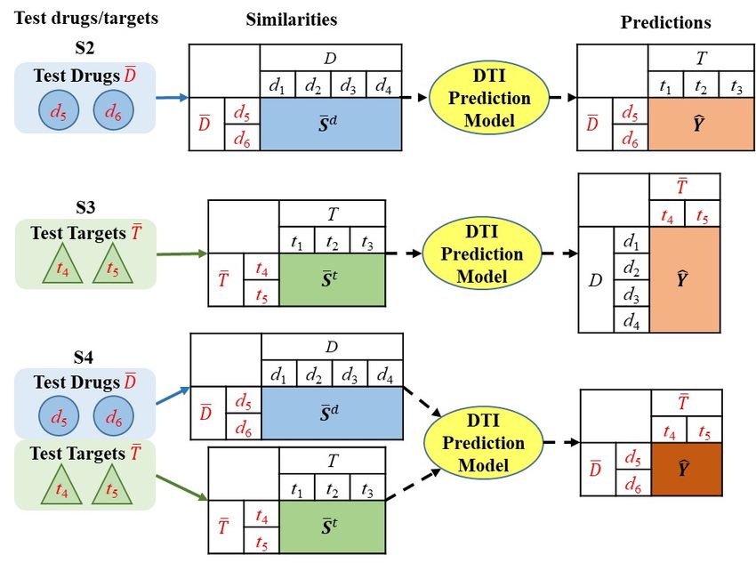
2                                                                    Bin Liu et al.

diction processes. We also propose a series of ensemble methods that employ
diverse sampling strategies and could be coupled with WkNNIR as well as any
other DTI prediction method to improve performance. Experimental results
over five benchmark datasets demonstrate the effectiveness of our approaches
in predicting drug-target interactions. Lastly, we confirm the practical predic-
tion ability of proposed methods to discover reliable interactions that were not
reported in the original benchmark datasets.
Keywords Drug-target interactions · Nearest neighbor · Interaction
recovery · Local imbalance · Ensemble learning

1 Introduction

Prediction of drug-target interactions (DTIs) is fundamental to the drug dis-
covery process [1, 2]. However, the identification of interactions between drugs
and specific targets via wet-lab (in vitro) experiments is extremely costly,
time-consuming, and challenging [3, 4]. Computational (in silico) methods
can efficiently complement existing in vitro activity detection strategies, lead-
ing to the identification of interacting drug-target pairs and accelerating the
drug discovery process.
     In the past, computational approaches identified DTIs mainly based on
known ligands for targets [5] or 3D protein structures [6]. However, these
methods suffer from two limitations. Firstly, they would collapse when the
required information (ligand-related information or 3D protein structures) is
unavailable. Secondly, they are built on only one kind of information. Re-
cently, chemogenomic approaches have attracted extensive interest, because
they integrate both drug and target information into a unified framework [1]
(e.g. chemical structure information related to drugs and genomic information
related to target proteins). Such information is often obtained via publicly
available databases.
     Popular chemogenomic approaches rely on machine learning algorithms,
which have been widely employed for DTI prediction tasks due to their verified
effectiveness [7]. There are several machine learning strategies to handle DTI
prediction [1]. Here, we focus on neighborhood approaches. These are typically
straightforward and effective methods that are based on similarity functions
[8]. Albeit rather simple, they are very promising. For instance, neighborhood
information is often used to regularize matrix factorization tasks, leading to
powerful DTI prediction methods [9]. Drug-drug similarities based on chemical
structure and target-target similarities based on protein sequence are the most
common types of information employed in DTI prediction tasks [1].
     Many of the existing similarity-based methods follow the transductive
learning scheme [9–14], where test pairs are presented and used during the
training process. Every time new pairs arrive, the learning model has to be
re-trained in order to perform predictions for them. This is computationally
inefficient and substantially affects the scalability of such models, especially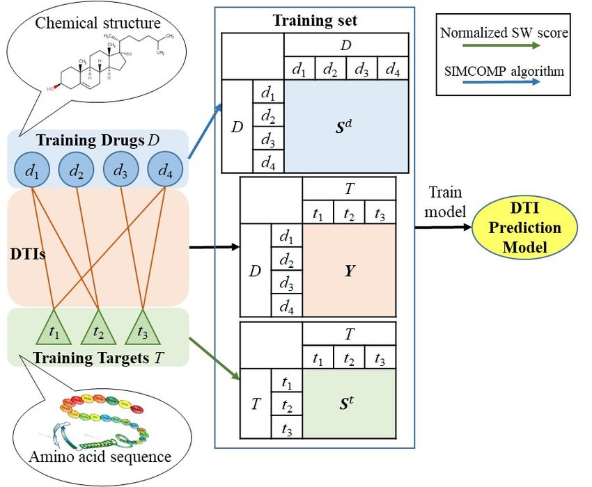
DTI Prediction via an Ensemble of WkNNIR                                      3

in cases where not all test pairs of drugs and targets can be gathered in ad-
vance. On the other hand, an inductive model is built upon a training dataset
consisting of a drug set, a target set and their interactivity, and can pre-
dict any unseen drug-target pairs without re-training. Therefore, we employ
similarity-based approaches following the inductive learning scheme, which is
more flexible and effective to perform predictions for newly arrived test pairs.
    Furthermore, many false negative drug-target pairs are typically included
in DTI training sets. These drug-target pairs are actually interacting, but the
interactions have not yet been reported (detected) due to the complex and
costly experimental verification process [15–17]. Hereafter, these interactions
shall be called missing interactions. When we treat the unverified DTIs as
non-interacting, we inevitably lose valuable information and introduce noise
to the data. Therefore, exploiting possible missing interactions is crucial for
the DTI prediction approach [15, 18].
    In DTI prediction, there are four main prediction settings. These include
predictions for: unseen pairs of training (known) drugs and targets (S1), pairs
of test (new) drugs and training targets (S2), pairs of test (new) targets and
training drugs (S3), and pairs of test (new) drugs and test (new) targets (S4).
Compared to S1, which only considers pairs consisting of known drugs and
targets, the other three settings that focus on predicting interactions for new
drugs and/or new targets are more difficult, because they relate to the cold-
start problem where interacting information of new drugs (targets) is unavail-
able [18]. This paper focuses on these three (S2, S3, S4) more challenging
settings.
    S4 is substantially more arduous than S2 and S3, as the bipartite com-
ponents of test pairs are new in S4. Many methods, especially most nearest
neighbor based ones [19, 11, 16], either cannot be applied or show a major drop
in prediction performance when it comes to S4. An existing neighborhood-
based approach designed for S4 specifically [20], can not perform predictions
in S2 and S3. Therefore, there is a lack of neighborhood-based DTI prediction
methods that can successfully handle each and every one of S2, S3, and S4.
Such methods are useful when the prediction setting of interest is unknown at
training time.
    We address DTI prediction with an emphasis on new drugs (S2), new tar-
gets (S3), and pairs of new drugs and new targets (S4). First, the formulation
of the inductive DTI prediction task that aims to perform predictions for any
unseen drug-target pair is defined and its differences with the transductive one
are clarified. Next, we propose a neighborhood-based DTI prediction method
called Weighted k-Nearest Neighbor with Interaction Recovery (WkNNIR).
The proposed method can deal with all prediction settings, as well as effec-
tively handle missing interactions. Specifically, WkNNIR detects neighbors of
test drugs, targets, and drug-target pairs to estimate interactions in S2, S3,
and S4, respectively. It updates the original interaction matrix based on the
neighborhood information to mitigate the impact of missing interactions. In
addition, WkNNIR exploits the concept of local class imbalance [21] to weigh
drug and target similarities, which boosts interaction recovery and prediction.
4                                                                    Bin Liu et al.

    Furthermore, we propose three ensemble methods to further improve the
performance of WkNNIR and other DTI prediction methods. These methods
follow a common framework that aggregates multiple DTI prediction mod-
els built upon diverse training sets deriving from the original training set by
sampling drugs and targets. They employ three different sampling strategies,
namely Ensemble with Random Sampling (ERS), Ensemble with Global im-
balance based Sampling (EGS), and Ensemble with Local imbalance based
Sampling (ELS). A short preliminary account of these three ensemble meth-
ods is given in [22].
    The performance of the proposed methods is evaluated on five benchmark
datasets. The obtained results show that WkNNIR outperforms other state-
of-the-art DTI prediction methods. We also show that ELS, EGS and ERS
are able to promote the performance of six different base models including
WkNNIR in all prediction settings, and ELS is the most effective one. Last,
we demonstrate cases where our methods succeed in discovering interactions
that had not been reported in the original benchmark datasets. The latter
highlights the potential of the proposed computational methods in finding
new interactions in the real world.
    The rest of this paper is organized as follows. In Section 2, existing DTI
prediction approaches are briefly presented. In Section 3, we define the formu-
lation of inductive DTI prediction and compare it with the transductive one.
The proposed neighborhood-based and ensemble methods are presented in
Sections 4 and 5, respectively. Experimental results and analysis are reported
in Section 6. Finally, we conclude our paper in Section 7.

2 Related Work

The fundamental assumption of similarity-based methods is that similar drugs
tend to interact with similar targets and vice versa [23]. Similarity-based meth-
ods can be divided into four types according to the learning method they
employ, namely Nearest Neighborhood (NN), Bipartite Local Model (BLM),
Matrix Factorization (MF) and Network Diffusion (ND).
    Nearest neighborhood based methods predict the interactions based on the
information of neighbors. Nearest Profile [19] infers interactions for a test drug
(target) from only its nearest neighbor in the training set. Weighted Profile
(WP) [19] integrates all interactions of training drugs (targets) by weighted
average to make predictions. Weighted Nearest Neighbor (WNN) [11] sorts all
training drugs (targets) based on their similarities to the test drug (target) in
descending order and assigns the weight of each training drug (target) accord-
ing to its rank. In WNN, interactions of training drugs (targets) whose weights
are larger than a predefined threshold are considered to make predictions. The
Weighted k-Nearest Known Neighbor (WKNKN) [16] was initially proposed
as a pre-processing step that transforms the binary interaction matrix into
an interaction likelihood matrix, while it can estimate interactions for test
drug (target) based on k nearest neighbors of training drugs (targets) as well.
DTI Prediction via an Ensemble of WkNNIR                                       5

The Similarity Rank-based Predictor [24] predicts interactions for test drug
(target) based on the likelihood of interaction and non-interaction obtained
by similarity ranking. All the above NN methods are restricted to the S2 and
S3 settings. In [20], three neighborhood-based methods, namely individual-to-
individual, individual-to-group, and nearest-neighbor-zone, designed specifi-
cally for predicting interactions between test drug and test target (S4) are
proposed. Furthermore, the well-known neighborhood-based multi-label learn-
ing method MLkNN [25] is employed for drug side effect prediction [26]. In
[15], MLkNN with Super-target Clustering (MLkNNSC) takes advantage of
super-targets that are constructed by clustering the interaction profiles of tar-
gets.
    BLM methods build two independent local models for drugs and targets,
respectively. They integrate the predictions of the two models to obtain the
final scores of test interactions. The first BLM method is proposed in [27],
where a support vector machine is employed as the base local classifier. Fur-
thermore, regularized least squares (RLS) formalized as kernel ridge regression
(RLS-avg) and RLS using Kronecker product kernel (RLS-kron) are two other
representative BLM approaches that process drug and target similarities as
kernels [28]. One weakness of the above BLM approaches is that they cannot
train local models for unseen drugs or targets. To address this issue, BLM-NII
[10], which is based on RLS-avg, introduces a step to infer interactions for
test drugs (targets) based on training data. Analogously, GIP-WNN [11] ex-
tends RLS-kron by adding the WNN process to estimate the interactions for
test drugs (targets). In Advanced Local Drug-Target Interaction Prediction
(ALADIN) [17], the local model is a k-Nearest Neighbor Regressor with Error
Correction (ECkNN) [29], which corrects the error caused by bad hubs. Such
hubs are often located in the neighborhood of other instances but have different
labels from those instances. Generally, BLM can predict interactions for test
drug-target pairs via a two-step learning process [30, 31], i.e. the interactions
between test drugs (targets) and training targets (drugs) are estimated first,
then two models based on those predictions are built to estimate interactions
between test drugs and test targets.
    MF methods deal with DTI prediction by factorizing the interaction ma-
trix into two low-rank matrices which correspond to latent features of drugs
and targets, respectively. Kernelized Bayesian Matrix Factorization with Twin
Kernels (KBMF2K) [32] and Probabilistic Matrix Factorization (PMF) [33]
conduct matrix factorization based on probability theory. KBMF2K follows a
Bayesian probabilistic formulation and PMF leverages the probabilistic linear
model with Gaussian noise. Collaborative Matrix Factorization (CMF) [34] is
applied to DTI prediction via adding low-rank decomposition regularization on
similarity matrices to ensure that latent features of similar drugs (targets) are
similar as well. In [12], soft weighting based self-paced learning is integrated
into CMF to avoid bad local minima caused by the non-convex objective func-
tion and achieve better generalization. Weighted Graph Regularized Matrix
Factorization (WGRMF) [16] performs graph regularization on latent features
of drugs and targets to learn a manifold for label propagation. Neighborhood
6 Bin Liu et al.
Regularized Logistic Matrix Factorization (NRLMF) [9] combines the typical
matrix factorization with neighborhood regularization in a unified framework
to model the probability of DTIs within the logistic function. Dual-Network
Integrated Logistic Matrix Factorization (DNILMF) [35], is an extension of
NRLMF that utilizes diffused drug and target kernels instead of similarity
matrices for the logistic function. MF approaches usually comply with the
transductive learning scheme.
Network-based inference (NBI) [36] applies network diffusion on the DTI
bipartite network leveraging graph-based techniques to predict new DTIs. This
approach uses only the interactions between drugs and targets. Domain Tuned-
Hybrid (DT-Hybrid) [37] and Heterogeneous Graph Based Inference (HGBI)
[38] extends NBI via incorporating drug-target interactions, drug similarities
and target similarities to the diffusion of the heterogeneous network. Apart
from network inference, random walk [39], probabilistic soft logic [40], and
finding simple path [41] are three other approaches that can be applied to the
heterogeneous DTI network to predict interactions. All of the ND methods are
transductive, as the network diffusion step should be recomputed if new drugs
or new targets are added in the heterogeneous network.
Apart from using similarities, there are methods that treat interaction pre-
diction as a classification task, building binary or multi-label classifiers over
input feature sets. In [42], traditional ensemble tree strategies, such as random
forests (RF) [43] and extremely randomized trees (ERT) [44], are extended to
the bi-clustering tree setting [45]. Another example is AGHEL [46], which is a
heterogeneous ensemble approach integrating two different classifiers, namely
RF and XGBoost [47]. Moreover, three tree-based multi-label classifiers which
incorporate various label partition strategies to effectively capture the cor-
relations among drugs and targets are proposed for DTI prediction in [48].
Furthermore, delivering low dimensional drug and target embeddings from a
DTI network using graph embedding [49, 14] or path category based extraction
techniques [50, 51, 13] has been shown very effective. However, these methods
are utilized in a transductive setting.
Finally, we briefly present approaches dealing with the issue of missing in-
teractions. The DTI prediction task with missing interactions can be treated as
a Positive-Unlabeled (PU) learning problem [52], where the training data con-
sists of positive and unlabeled instances and only a part of positive instances
are labeled. Several methods mentioned above discover missing interactions
by using matrix completion techniques [34, 9]. Others construct super-targets
containing more interacting information [15], correct possible missing inter-
actions [17], and recover interactions as a pre-processing step [16]. Similar to
the idea of interaction recovery, Bi-Clustering Trees with output space Recon-
struction (BICTR) [18] utilizes NRLMF to restore the training interactions on
which an ensemble of Bi-clustering trees [42] is built. In [53, 54], traditional PU
learning algorithms, such as Spy and Rocchio, are employed to extract reliable
non-interacting drug-target pairs. Based on a more informative PU learning
assumption that interactions are not missing at random, a probabilistic model
without bias to labeled data is proposed in [55].DTI Prediction via an Ensemble of WkNNIR 7
3 Inductive DTI Prediction
In this section, the formulation of similarity based DTI prediction in an induc-
tive learning scheme is presented. Then, the comparison between the inductive
and transductive settings for the DTI prediction task is given.
3.1 Formulation
In this part, we define the inductive DTI prediction problem, as well as the
training and estimation procedures of a DTI prediction model in inductive
learning, where the drug and target similarities are utilized as input informa-
tion.
Let D = {di }ni=1 be the training drug set containing n drugs, where each
drug is a compound described by its chemical structure. Let T = {ti }m i=1 be
the training target set consisting of m targets, where each target is a protein
represented by its amino acid sequence. There is a set of known interactions
between drugs in D and targets in T . Fig.1(a) illustrates the process of train-
ing an inductive model. Initially, to cater for a similarity-based DTI prediction
model, the drug similarity matrix S d ∈ Rn×n and the target similarity ma-
trix S t ∈ Rm×m are computed, where Sij d
is the similarity between di and dj ,
t
and Sij is the similarity between ti and tj . In this paper, drug similarities are
computed by SIMCOMP algorithm [56], which assesses the common chemical
structure of two drugs, and target similarities are calculated by using the nor-
malized Smith-Waterman (SW) score [57], which evaluates the shared amino
acid sub-sequence of two targets. In addition, DTIs are represented with an
interaction matrix Y ∈ {0, 1}n×m , where Yij = 1 if di and tj are known to
interact with each other and Yij = 0 indicates that di and tj either actually
interact with each other but their interaction is undetected, or di and tj do
not interact. An inductive DTI prediction model is built based on a training
set consisting of D, T , S d , S t and Y .
In the prediction phase, as discussed in the introduction, we distinguish
three settings of DTI prediction, according to whether the drug and target
involved in the test pair are included in the training set or not. In particular:
– S2: predict the interactions between test drugs D̄ and training targets T .
– S3: predict the interactions between training drugs D and test targets T̄ .
– S4: predict the interactions between test drugs D̄ and test targets T̄ .
where D̄ = {du }n̄u=1 is a set of test drugs disjoint from the training drug set
(i.e. D̄ ∩ D = ∅), and T̄ = {tv }m̄
v=1 is a set of test targets disjoint from T .
The prediction procedure is shown in Fig. 1(b). In all prediction settings,
the similarities between test drugs (targets) and training drugs (targets), re-
quired by the similarity-based model, are firstly computed. Next, the learned
DTI prediction model receives these similarities to perform predictions for the
corresponding test drug-target pairs. In S2, given a set of test drugs D̄, the
similarities between D̄ and D (S̄ d ∈ Rn̄×n ) computed by the SIMCOMP al-
gorithm are input to the model, and the predictions are a real-valued matrix8 Bin Liu et al.
Ŷ ∈ Rn̄×m indicating the confidence of the affinities between test drugs and
training targets. Similarly in S3, the normalized SW score is employed to cal-
culate the similarities between T̄ and T (S̄ t ∈ Rm̄×m ), upon which the model
outputs a prediction matrix Ŷ ∈ Rn×m̄ . In S4, both S̄ d and S̄ t are computed,
and the prediction matrix is Ŷ ∈ Rn̄×m̄ .
3.2 Comparison between Inductive and Transductive Settings
In the transductive learning scheme, the model is learned for the purpose of
predicting specific test pairs. Fig. 1(c) describes the training and prediction
processes of a model in the transductive setting dealing with S4. Both training
and test drugs (targets) are available in the learning phase of a transductive
model. Given that D̃ = D ∪ D̄ and T̃ = T ∪ T̄ , one would first compute the
extended drug and target similarity matrices for D̃ and T̃ , respectively:
" # " #
> >
d Sd S¯d t S t S̄ t
S̃ = ¯d S̃ = ¯t (1)
S̄ d S̄ S̄ t S̄
where S̄ ¯ d ∈ Rn̄×n̄ (S̄¯ t ∈ Rm̄×m̄ ) stores similarities between test drugs (tar-
gets). In addition, the interaction matrix is extended to Ỹ ∈ {0, 1}(n+n̄)×(m+m̄) ,
where the rows and columns of Ỹ corresponding to test drugs and targets con-
tain “0”s. The transductive model is trained upon the input consisting of D̃,
T̃ , S̃ d , S̃ t and Ỹ , and could perform predictions for the specific test pairs
included in the input once it has been built. The processes of the transductive
model handling S2 and S3 are similar with S4, except for that no test target
and drug are used in S2 and S3, respectively (e.g in S3, D̄ = ∅, the drug
similarity matrix is S t and the interaction matrix is [Y , 0]).
The difference between the inductive and transductive settings relies on
their input information and the predicting ability of the model. On one hand,
an inductive model is built in the training phase, using similarity and interac-
tion matrices referring to training drugs and targets. After the completion of
this process, it can perform predictions for any setting (S2, S3, S4) and any
unseen pairs. On the other hand, a transductive model is built upon both the
information of the training set and the similarities of the test drugs and/or
targets. Hence, it can provide predictions only for these specific test pairs and
cannot generalize to unseen test data. If a transductive model needs to predict
the interaction of another unseen drug-target pair different to the one included
in the training process, it should be re-trained, incorporating the information
corresponding to the unseen test pair. This is extremely demanding, especially
when it comes to large scale data. Therefore, in this paper, we focus on the
inductive setting.DTI Prediction via an Ensemble of WkNNIR 9
(a) Training phase of an inductive model
(b) Prediction phase of an inductive model
(c) The training and prediction procedure of a transductive model dealing with S4
Fig. 1: Comparison between inductive and transductive settings10 Bin Liu et al.
4 WKNNIR
In this section, we first propose the Weighted k-Nearest Neighbor (WkNN)
as a comprehensive nearest neighbor based approach that could handle all
prediction settings. Next, the local imbalance is introduced to measure the
reliability of similarity matrices. Lastly, WkNNIR, which incorporates inter-
action recovery and local imbalance driven similarity weighing into WkNN, is
presented.
4.1 WkNN
Neighborhood-based methods predict the interactions of test drugs (S2) or
test targets (S3) by aggregating the interaction profiles of their neighbors
[19, 11, 16]. The major limitation of these methods is that they cannot directly
predict interactions between test drugs and test targets (S4), as interactions
between test drugs (targets) and their neighbors are unavailable in the training
set. To overcome this drawback of existing methods, we propose WkNN.
WkNN employs the prediction function of WKNKN [16] to deal with S2
and S3 because of its simplicity and efficacy. WkNN is a lazy learning method
that does not have any specific training phase. Given a test drug-target pair
(du , tv ) belonging to the prediction setting S2 or S3, WkNN predicts their
interaction profiles based on the interactions of either k nearest training drugs
of du or k nearest training targets of tv as follows:
1 X 0
η i −1 S̄ui
d
Yiv , if du ∈
/ D and tv ∈ T
z
d
u
di ∈Ndku
Ŷuv = (2)
1 X j 0 −1 t
η S̄vj Yuj , if du ∈ D and tv ∈ /T
ztv
k
tj ∈Ntv
In Eq.(2), Ndku (Ntkv ) corresponds to k nearest neighbors of du (tv ) which are
retrieved by choosing k training drugs (targets) having k largest values in u-th
row of S̄ d (v-th row of S̄ t ) and sorting the selected k drugs (targets) in the
descending order according to their similarities to du (tv ). Moreover, di (tj ) is
the i0 -th (j 0 -th) nearest neighbor of du (tv ), i.e. i0 (j 0 ) is the index of di (tj )
in Ndku (Ntkv ), η ∈ [0, 1] is the decay coefficient shrinking the weight of further
d t
P P
neighbors, and zdu = di ∈N k S̄ui and ztv = tj ∈N k Svj are normalization
du tv
terms.
To make predictions for pairs of test drugs and test targets (S4), WkNN fol-
lows the tetrad rule: when a drug interacts with a target, another similar drug
probably interacts with another similar target [40]. For the sake of adapting to
the tetrad rule, WkNN considers similar drug-target pairs instead of similar
drugs or targets. We define the neighbors of a test drug-target pair (du , tv ) as
Ndku tv = {(di , tj )|di ∈ Ndku , tj ∈ Ntkv }. Although the direct way to find neigh-
bors of a drug-target pair is to search all nm drug-target combinations, ourDTI Prediction via an Ensemble of WkNNIR 11
definition shrinks the search space to n + m leading to increased efficiency.
As in [28, 11], we define the similarity between two drug-target pairs as the
product of the similarity of two drugs and the similarity of two targets, i.e.
d t
the similarity of (du , tv ) and (di , tj ) is S̄ui S̄vj . Thus, the prediction function
of WkNN for S4 is:
1 X 0 0
−2
Ŷuv = η i +j d t
S̄ui S̄vj Yij (3)
zuv
(di ,tj )∈Ndku tv
d t
P
where the normalization term zuv is equal to (di ,tj )∈N k S̄ui S̄vj . The weight
d u tv
in Eq.(3) consists of two parts: the first one corresponds to the decay coeffi-
cient, where the exponent is determined by the index of di in Ndku (i0 ) and
the index of tj in Ntkv (j 0 ) simultaneously, and the second one is the similarity
between the test pair and its neighbor.
4.2 Local Imbalance
The concept of local imbalance concerns the label distribution of an instance
within the local region, playing a key role in determining the difficulty of a
dataset to be learned [21]. Concerning DTI data that contain two kinds of
similarities, the local imbalance can be assessed in both drug space and target
space.
Firstly, we define the drug-based local imbalance. The local imbalance of a
drug di for target tj is measured as the proportion of Ndki having the opposite
interactivity to tj as di :
d 1 X
Cij = JYhj 6= Yij K (4)
k k
dh ∈Nd
i
d
where Cij ∈ [0, 1] and JxK is the indicator function that returns 1 if x is true
d
and 0 otherwise. The larger the value of Cij , the fewer the drugs in the local
region of di having the same interactivity to tj , and the higher the local im-
balance of di for tj based on drug similarities. In the ideal case, similar drugs
share the same interaction profiles (i.e. interact with the same targets), render-
ing DTI prediction a very simple task. However, there are several cases, where
similar drugs interact with different targets, which makes DTI prediction more
d
challenging. Therefore, we employ local imbalance Cij to assess the reliabil-
d
ity of similarities between di and other training drugs. Specifically, lower Cij
indicates more reliable similarity information.
Likewise, we calculate the local imbalance of tj for di based on the targets
as:
t 1 X
Cij = JYih 6= Yij K (5)
k k
th ∈Nt
j12 Bin Liu et al.
4.3 WkNNIR
The existence of missing interactions (not yet reported) in the training set
can lead to biased DTI prediction models and an inevitable accuracy drop. To
address this issue, we propose WkNNIR, which couples WkNN with interac-
tion recovery to perform predictions upon the completed interaction matrix.
Moreover, in S4, where both drug and target similarities are used to perform
predictions, WkNNIR has the advantage that the importance (weight) of drug
and target similarities is differentiated depending on their local imbalance.
Firstly, WkNNIR computes recovered interactions, which replace the origi-
nal interactions in the prediction phase. Based on the assumption that similar
drugs interact with similar targets and vice versa, missing interactions can
be completed by considering the interactions for neighbor drugs or targets.
There are two ways to recover the interaction matrix: one on the drug side
and another on the target side. The drug side recovery is conducted row-wise,
where each row of Y is recovered by the weighted average of the neighbor rows
identified by drug similarities. The drug-based recovery interaction matrix Y d
is:
1 X h0 −1 d
Yi·d = η Sih Yi· , i = 1, · · · , n (6)
zdi k
dh ∈Nd
i
where h0 is the index of dh in Ndki , and zdi = d
P
dh ∈Ndk Sih . The target-based
i
recovery interaction matrix Y t is obtained by reconstructing Y column-wise:
1 X l0 −1 t
Y·jt = η Slj Y·j , j = 1, · · · , m (7)
ztj k
tl ∈Nt
j
where l0 is the index of tl in Ntkj and ztj = t
P
tl ∈Ntk Slj .
j
However, Y d (Y t ) exploits only one kind of similarity and neglects the
other one. To address this issue, we combine these two recovered interaction
matrices into a complementary one that incorporates the recovery informa-
tion from both drug and target views. Besides, interactions restored via more
reliable similarity measures tend to be more credible. Therefore, instead of
treating Y d and Y t equally, we distinguish the effectiveness of different re-
covered interaction matrices according to the local imbalance of the similarity
used in the recovery process.
The interacting pair (di , tj ) with lower drug-based local imbalance indicates
that di is close to other drugs interacting with tj in the drug space, and
therefore the recovered interactions inferred from the pair are more reliable
in the drug view. Hence, we define the weight of recovered interaction Yijd
according to the average local imbalance of interacting pairs that are used to
estimate Yijd :
d
P
dh ∈Ndk Chj Yhj
d i
Wij = exp(− P ) (8)
dh ∈N k Yhj
diDTI Prediction via an Ensemble of WkNNIR 13
Similarly, the weight of recovered interaction Yijt is computed as:
t
P
tl ∈Ntk Clj Yil
t j
Wij = exp(− P ) (9)
tl ∈N k Yil tj
The higher the weight, the more reliable the recovered interaction. By weighted
aggregation of the Yd and Yt , we obtain the final recovered interaction matrix
Y dt ∈ Rn×m :
Wijd Yijd + Wijt Yijt
Yijdt = , i = 1, · · · , n; j = 1, · · · , m (10)
Wijd + Wijt
By multiplying with the local imbalance-based weight, interactions recovered
by more reliable similarities have more influence on Y dt . The values in Y dt
are in the range of [0,1]. Furthermore, because “1”s in Y denotes reliable in-
teractions that do not need any update, a correction process is applied to the
reconstructed interaction matrix to ensure the consistency of known interac-
tions:
Y dt = max{Y dt , Y } (11)
where max is the element wise maximum operator.
In the prediction phase, the estimated interaction between drug du and
target tv is calculated as:
1 X i0 −1 d dt
η S̄ui Yiv , if du ∈
/ D and tv ∈ T
zdu di ∈Ndku
1 X 0
η j −1 S̄vj
t dt
Yuj , if du ∈ D and tv ∈ /T
ztv
Ŷuv = tj ∈Ntv k (12)
1
X 0 0
η i +j −2 (S̄ui
d rd t rt dt
) (S̄vj ) Yij
zuv k
(di ,tj )∈Ndu tv
if du ∈ / D and tv ∈ /T
where rd = min{1, Lduv /Ltuv } and rt = min{1, Ltuv /Lduv } are the coefficients
controlling the weights of drug similarities and target similarities respectively.
The smaller rd is, the largerPdrug similarities become, as bothP similarities and
rd are between [0,1]. Lduv = (di ,tj )∈N k Cij d
Yij and Ltuv = (di ,tj )∈N k Cij t
Yij
d u tv d u tv
are the sum of drug-based and target-based local imbalance of neighbor pairs
of (du , tv ) respectively. Compared with Eq.(2) and (3) in WkNN, there are
two improvements made in WkNNIR. The first one is the utilization of re-
covered interaction matrix with more sufficient interaction information. The
second advantage of WkNNIR is the more reliable similarity assessment via
local imbalance by using rd and rt in S4.
The workflow of WkNNIR is presented in Fig. 2. In the training phase,
it sequentially computes Ndki for each training drug di ∈ D, drug-based local14 Bin Liu et al. imbalance matrix C d , drug-based recovery interaction matrix Y d and W d representing weights of Y d , using the training set. Similar variables relating to targets, namely Ntkj , C t , Y t and W t , are calculated too. Then, the final interaction matrix Y dt incorporating the recovered interactions in both Y d and Y t is obtained according to Eq.(10) and Eq.(11). In the prediction phase, given test drug and/or target similarities, the estimated interaction matrix Ŷ is obtained based on the recovered interaction matrix Y dt according to Eq.(12). Fig. 2: The workflow of WkNNIR. Solid and dashed arrows denote steps in the training and prediction phases, respectively. 5 Ensembles of DTI Prediction Models Ensemble methods integrate multiple models that solve the same task, and therefore reduce the generalization error of single models. In this section, we propose three ensemble methods, namely ERS, EGS and ELS, which employ random sampling, global imbalance based sampling, and local imbalance based sampling respectively. The three proposed ensemble methods follow the same framework and can be applied to any DTI prediction method to further im- prove its accuracy. We firstly introduce the ensemble framework and then describe the sampling strategies used in each method.
DTI Prediction via an Ensemble of WkNNIR                                                     15

5.1 Ensemble Framework

The proposed ensemble framework learns multiple models based on diverse
sampled training subsets. To adapt it to the DTI prediction task, the proposed
framework needs to be modified in the following aspects: adjusting the sampled
training subsets generation in the training phase as well as adding dynamic
ensemble selection and similarity vector projection processes in the prediction
phase.
    The pseudo code of training an ensemble model is shown in Algorithm 1. In
the training phase, the sampling probabilities for drugs and targets, denoted
     d     n       t
Pnp ∈dR and p P
as                   ∈ Rm , are initially computed (Algorithm 1, line 2-3), where
                       m    t
   i=1 pi = 1 and      j=1 pj = 1. The calculation of the sampling probabilities
is different in each of the three methods and will be illustrated in Section 5.2.
Then, q base models are trained iteratively. For the i-th base model, the nR
sized drug subset Di is sampled from D without replacement according to
pd (Algorithm 1, line 5), i.e. drugs with larger sampling probability have a
greater chance to be added to Di , where R is a user-specified sampling ratio
controlling the number of selected drugs. In a similar way, the mR sized target
subset T i is derived from T based on pt (Algorithm 1, line 6). In the next step,
based on the Di and T i , we form a training subset which consists of a drug
similarity sub-matrix S di retaining similarities between drugs in Di , a target
similarity sub-matrix S ti preserving the similarities between targets in T i and
an interaction sub-matrix Y i storing interactions involving both Di and T i
(Algorithm 1, line 7). Finally, the base model Mi is trained on the obtained
training subset (Algorithm 1, line 8).

 Algorithm 1: Training Ensembles of DTI Prediction Models
     input : training drug set: D, training target set: T , drug similarity matrix: S d ,
                target similarity matrix: S t , interaction matrix: Y , sampling ratio: R,
                ensemble size: q
     output: ensemble model: M , drug subsets: D0 , target subsets: T 0
 1   M, D0 , T 0 ← ∅ ;
 2   Calculate the sampling probability for drugs pd ;
 3   Calculate the sampling probability for targets pt ;
 4   for i ← 1 to q do
 5       Di ← sample nR drugs from D based on pd ;
 6       T i ← sample mR targets from T based on pt ;
 7       Construct training subset S di , S ti , Y i based on Di and T i ;
 8       Mi ← Train(S di , S ti , Y i , Di , T i ) ;
 9       M ← M ∪ Mi ;
10       D0 ← D0 ∪ Di ;
11       T0 ← T0 ∪ Ti ;
12   return M, D0 , T 0 ;

    The prediction process of the ensemble framework is illustrated in Algo-
rithm 2. The input similarity sdu (stv ) is equivalent to Su·
                                                           d    t
                                                              (Sv· ) if du ∈ D
16 Bin Liu et al.
d t
(tv ∈ T ), and S̄u· (S̄v· ) otherwise. Dynamic ensemble selection takes place
first if the test drug-target pair (du , tv ) follows the condition of S2 or S3.
Specifically, when (du , tv ) follows S2, Mi is discarded if test target tv ∈ / Ti
(Algorithm 2, line 2-4). Compared with other base models involving tv in the
training process, Mi misses the information of interaction regarding tv and usu-
ally leads to a lower prediction accuracy for (du , tv ). Analogously, the models
whose corresponding training drug subset does not contain du are discarded if
(du , tv ) follows S3 (Algorithm 2, line 5-7). Dynamic ensemble selection is not
applied to S4 (du ∈ / D and tv ∈ / T ), because both du and tv are new emerging
drugs and targets for all base models in S4. In the next steps, all retained
base models give their prediction, which are eventually averaged to obtain the
final predicted score Ŷuv (Algorithm 2, line 9-14). It should be noticed that
there are two projection steps to ensure the similarity vectors of the drug and
target in the test pair fit the input of each base model (Algorithm 2, line 10-
11). As each base model is trained based on a subset of drugs and targets,
the similarity vector for du and tv should be projected to the low dimensional
space characterized by the drug and target subset used in the corresponding
base model. Specifically, the projection of sdu on Di maintains the similarities
between du and drugs in Di and deletes other elements in sdu . For example,
given a similarity vector [0.1, 0.2, 0.3, 0.4, 0.5], its projection on drug subset
{d1 , d2 , d4 } is [0.1, 0.2, 0.4].
Algorithm 2: Predicting of Ensemble DTI Prediction
input : ensemble of DTI prediction model: M , drug subsets: D0 , target subsets:
T 0 , training drug set: D, training target set: T , test drug-target pair:
(du ,tv ), similarity of du to D: sdu , similarity of tv to T : stv
output: predicting interaction between du and tv : Ŷuv
1 for i ← 1 to |M | do /* Dynamic ensemble selection */
2 if du ∈
/ D and tv ∈ T then /* S2 */
3 if tv ∈ / Ti then
4 M ← M − Mi ;
5 if du ∈ D and tv ∈
/ T then /* S3 */
6 if du ∈
/ Di then
7 M ← M − Mi ;
8 Ŷuv ← 0 ;
9 for i ← 1 to |M | do /* Predicting */
10 s0d d
u ← Project su on D ;
i
11 sv0t ← Project stv on T i ;
12 Yuv0 ← Predict(M , s0d , s0t , d , t ) ;
i u v u v
13 Ŷuv ← Ŷuv + Yuv0 ;
14 Ŷuv ← Ŷuv /|M | ;
15 return Ŷuv ;DTI Prediction via an Ensemble of WkNNIR 17
5.2 Sampling Probability
Sampling probabilities determine the opportunity of each drug and target
being used to train base models, which play a key role in the proposed ensemble
framework. As we mentioned before, the three proposed ensemble methods
employ different sampling probabilities.
ERS adopts the sampling probabilities following the uniform distribution,
i.e. pdi = 1/n and ptj = 1/m, where i = 1, 2, ...n and j = 1, 2, ...m. In this way,
each drug and target has an equal chance to be selected.
In DTI data, interacting drug-target pairs are heavily outnumbered by
non-interacting ones, resulting in an imbalanced distribution within the global
interaction matrix. To relieve this global imbalance, EGS forms training sub-
sets by biasing the sampling process to include drugs and targets having more
interactions. Moreover, another reason for emphasis on drugs and targets with
dense interactions is that they are more informative than others with fewer
interactions. In EGS, the sampling probability of each drug (target) is propor-
tional to the number of its interactions:
Pm
d
σ + j=1 Yij
pi = Pn Pm , i = 1, 2, ...n
nσ + h=1 j=1 Yhj
Pn (13)
t σ + i=1 Yij
pj = Pn Pm , j = 1, 2, ...m
mσ + i=1 h=1 Yih
where σ is a smoothing parameter. By using Eq. (13), the drugs and targets
with more interactions are more likely to be selected in the sampling procedure.
Apart from the global imbalance, the local imbalance could also be used to
d
assess the importance of that drug (target). According to Eq.(4), higher Cij
means that di is surrounded by more drugs that have opposite interactivity to
tj . In such cases, correctly predicting Yij using drug similarities would be dif-
ficult. By accumulating the local imbalance (difficulty) of di for all interacting
targets, we arrive at the local imbalance based importance of di :
m
X
LIid = d
Cij JYij = 1K (14)
j=1
Pm
LIid is a weighted sum version of j=1 Yij , where the interaction which is
difficult to be predicted correctly is assigned a higher weight. Compared with
EGS only counting the interactions of drugs, Eq. (14) emphasizes on drugs
having more difficult interactions.
Similarly, the local imbalance based importance of tj is defined as:
n
X
LIjt = t
Cij JYij = 1K (15)
i=1
Based on the definition of local imbalanced based importance, the key idea in
ELS is that it encourages more difficult drugs and targets to be learned by more18 Bin Liu et al.
base models, reducing thereby the corresponding error to the greatest extent
possible. In ELS, the sampling probability is proportional to the corresponding
local imbalance based importance:
σ + LIid
pdi = Pn , i = 1, 2, ...n
nσ + h=1 LIhd
(16)
σ + LIjt
ptj = Pm , j = 1, 2, ...m
mσ + h=1 LIht
In addition, we exemplify the differences of three sampling probabilities in
Fig. 3. In ERS, all drugs have equal chance to be selected. EGS is more likely
to choose d3 , d4 and d5 that have more interacting targets. ELS will select
d1 with higher probability, because d1 is near (similar) to drugs (d2 and d3 )
having different interactions and is therefore more difficult to be learned than
other drugs.
Fig. 3: The differences of the three sampling probabilities. The top half shows
the drugs’ location (blue circles) and their interactions (light red rectangles) of
a dataset including five drugs and three targets. The table in the bottom half
lists the drug sampling probabilities computed by the three ensemble methods
on this dataset with σ = 0.1 and k = 2
6 Experiments
In this section, the datasets and the evaluation protocol used in the experi-
ments are presented firstly. Then, the predictive performance and parameterDTI Prediction via an Ensemble of WkNNIR 19
analysis of proposed WkNNIR and three ensembles are reported. Finally, newly
discovered interactions found by our methods are presented.
6.1 Dataset
Five benchmark DTI datasets are used in our empirical study. Four of them are
gold standard datasets originally provided by [19], of which each corresponds
to a target protein family, namely Nuclear Receptors (NR), G-protein cou-
pled receptors (GPCR), Ion Channel (IC) and Enzyme (E). The last dataset
(DB), obtained from [58], was derived from DrugBank [59]. Table 1 lists the
information about the five datasets. Sparsity is the proportion of interacting
drug-target pairs which indicates the global imbalance of the dataset. LI d and
LI t are the drug-based and target-based local imbalance of the whole dataset
respectively:
Pn Pm d
d i=1 j=1 Cij Yij
LI = Pn Pm (17)
i=1 j=1 Yij
Pn Pm t
t i=1 j=1 Cij Yij
LI = Pn Pm (18)
i=1 j=1 Yij
where k is the number of neighbors, which is set to 5. Smaller LI d (LI t ) values
indicate more reliable drug (target) similarities and easier S2 (S3) prediction
task.
Table 1: Statistic of DTI datasets
Dataset # Drugs # Targets # Interactions Sparsity LI d LI t
NR 54 26 90 0.064 0.658 0.764
GPCR 223 95 635 0.03 0.707 0.644
IC 210 204 1476 0.035 0.729 0.323
E 445 664 2926 0.01 0.737 0.35
DB 786 809 3681 0.006 0.653 0.528
6.2 Evaluation protocol
Three types of cross validation (CV) are conducted to examine the prediction
methods in three prediction settings, respectively. In S2, the drug wise CV is
applied where one drug fold along with their corresponding rows in Y are sep-
arated for testing. In S3, the target wise CV is utilized where one target fold
along with their corresponding column in Y are left out for testing. The block
wise CV, which splits a drug fold and target fold along with the interactions
between them (which is a sub-matrix of Y ) for testing and uses interactions20 Bin Liu et al.
between remaining drugs and targets for training, is applied to S4. Two rep-
etitions of 10-fold CV are applied to S2 and S3, and two repetitions of 3-fold
block wise CV which contains 9 block folds generated by 3 drug folds and 3
target folds are applied to S4.
The Area Under the Precision-Recall curve (AUPR) which heavily punishes
highly ranked false positive predictions [60] is used to evaluate the performance
of inductive DTI prediction approaches in our experiments. In addition, the
Wilcoxon signed rank test at 5% level is utilized to examine the statistically
significant difference between our methods and the compared ones.
In the experiments, we firstly compare the proposed WkNNIR with six
DTI prediction approaches, namely ALADIN [17], BICTR [18], BLM-MLkNN
[26, 30], BLM-NII [10], MLkNNSC [15], NRLMF [9], as well as WkNN which
is the baseline of WkNNIR without interaction recovery and local imbalance
weighting. All comparing methods except for BICTR either follow the trans-
ductive DTI prediction task or work for partial prediction settings. Therefore,
we extend those methods to handle the inductive DTI prediction problem and
all prediction settings as follows:
– ALADIN [17]: ALADIN works for S2 and S3 within the inductive scheme.
As a BLM approach, ALADIN could deal with S4 by using the two-step
learning strategy.
– BLM-MLkNN [26, 30]: An individual MLkNN model could only deal with
S2 and S3 following the inductive scheme. To deal with S4, the MLkNN is
embedded in the BLM and the two-step learning strategy is adopted.
– MLkNNSC [15]: MLkNNSC is initially proposed to predict interactions for
test drugs (S2) and test drug-target pairs (S4) and it could work as an
inductive approach directly. To handle S3 prediction setting, MLkNNSC
is extended via applying clustering for drugs to obtain super-drugs and
training MLkNN models for drugs and super-drugs, respectively.
– BLM-NII [10]: BLM-NNI is a transductive method and able to tackle all
prediction settings. To enable BLM-NNI to adapt the inductive DTI pre-
diction, we modify its training and prediction process by confining that
similarities for test drugs (targets) are available in prediction phase only.
– NRLMF [9]: NRLMF predicts interactions for S2, S3, and S4 in the trans-
ductive way. Similar to BLM-NII, NRLMF is altered to an inductive method
by excluding similarities for test drugs and targets from the input of the
training phase.
Moreover, BICTR trains an ensemble of bi-clustering trees on a reconstructed
interaction matrix which is completed by NRLMF, and the input of the tree-
ensemble model is the drug and target features. Hence, the similarities are
utilized as features in BICTR, i.e. the feature vector of a drug (target) is its
similarities to all training drugs (targets).
When it comes to ensemble methods i.e. ERS, EGS and ELS, four com-
paring DTI methods, namely ALADIN, BLM-NII, MLkNNSC, NRLMF and
the two proposed neighborhood based approaches (WkNN and WkNNIR) are
utilized as base model. We do not employ BICTR and BLM-MLkNN as baseDTI Prediction via an Ensemble of WkNNIR 21
model, because the former one is already an ensemble model and the latter
one is the worst method in most cases.
The parameter settings of compared and proposed methods are listed in
Table 2. The values for used parameters are selected by performing the inner
CV on the training set. Specifically, the 5-fold inner CV is applied to S2 and
S3, and the 2-fold inner CV is applied to S4 on GPCR, IC, E and DB datasets.
For NR dataset containing fewer drugs and targets, splitting NR into fewer
folds generates small-sized training sets that may vary the distribution of the
whole dataset during the inner CV procedure. This leads to the unreliability
of chosen optimal parameter settings. To avoid this issue, we apply the 10-fold
inner CV for S2 and S3 and the 3-fold inner CV for S4 on NR dataset.
Table 2: Parameter settings
Method Values or ranges of parameters
ALADIN #models=25, k ∈{1,2,3,5,7,9}, #features∈{10,20,50}
BICTR #trees=100, minimal # samples in leaf=1 (2) in S3 and S4 (S2)
BLM-MLkNN k ∈{1,2,3,5,7,9}
BLM-NII γ = 1, α ∈ {0, 0.1,...,1.0}, λ ∈ {2−5 , 2−4 , ..., 20 }
MLkNNSC cut-off threshold= 1.1, k ∈{1,2,3,5,7,9}
NRLMF c=5, k=5, r ∈ {50,100}, λt , λd , α, β ∈ {2−5 , 2−4 , ..., 20 }
WkNN k ∈{1,2,3,5,7,9}, η ∈ {0.1,0.2,...,1.0}
WkNNIR k ∈{1,2,3,5,7,9}, η ∈ {0.1,0.2,...,1.0}
ERS q = 30, R = 0.95
EGS q = 30, R = 0.95 σ = 1.0(0.1) for DB dataset (others)
ELS q = 30, R = 0.95, σ = 1.0(0.1) for DB dataset (others), k = 5
6.3 Results
In this part, the obtained results comparing the proposed WkNNIR and its
baseline WkNN to other competitors are presented and discussed. Next, the
results of the three proposed ensemble methods with six different base models
are reported.
Table 3 shows the AUPR results for the compared approaches in vari-
ous prediction prediction settings, where “*” following the numerical results
indicates that the corresponding method is statistically different from WkN-
NIR using Wilcoxon signed rank test at 5% level. WkNNIR achieves the best
average rank in all settings. It is significantly superior to other methods in
83/105 cases and does not suffer any significant losses from other competi-
tors. In addition, WkNNIR significantly outperforms WkNN in 13/15 cases,
demonstrating the effectiveness of the utilization of the interaction recovery
and local imbalance-based weights. Then, we investigate the results in each
prediction setting. In S2, WkNNIR is the best method on all datasets. WkNN
is the second best method and NRLMF comes next in most cases. In S3, for22 Bin Liu et al.
more difficult datasets (GPCR and DB having higher target-based local im-
balance), WkNNIR is the top method, while for easier datasets (IC and E
having lower target-based local imbalance) and the small-sized dataset (NR),
WkNNIR achieves comparable performance to the corresponding best method
without statistically significant difference. In S4, WkNNIR outperforms other
competitors on the first three datasets and is slightly inferior to WkNN on E
as well as BICTR on DB without significant difference. WkNN outperforms all
other six competitors on the first four datasets, which indicates the effective-
ness of our proposed neighbor pair based prediction function for S4. Overall,
WkNNIR surpasses the compared methods in S2 and S4 and is comparable
with state-of-the-art approaches in S3.
As is deducted from the obtained results, the three prediction settings,
namely S2, S3, and S4, are not equally challenging. In Table 3, AUPR results
of all methods in S4 are immensely lower than that in S2 and S3 on all datasets.
This shows that predicting interactions between test drugs and test targets is
the most challenging task. Comparing results in S2 and S3, we find that all
methods achieve higher AUPR in S3 than S2 on GPCR, IC, E and DB whose
LI t is lower than LI d . While the performance of all methods, except for BLM-
NII, in S3 is inferior to S2 on NR, whose LI t is higher than LI d . This indicates
that the difficulty of S2 and S3 could be estimated by comparing LI d and LI t ,
e.g. S2 is harder than S3 if LI d is higher than LI t , and vice versa. This also
verifies the effectiveness of the local imbalance to assess the reliability of drug
and target similarities.
As we previously stated, DTI datasets usually contain many missing in-
teractions, e.g. the four gold standard datasets only contain interactions dis-
covered before they were constructed (in 2007). To test the effectiveness of
WkNNIR on datasets with fewer missing interactions, we follow the procedure
described in [61] to build updated gold standard datasets that include more val-
idated interactions. Specifically, we add newly discovered interactions between
drugs and targets in the original datasets recorded in the up-to-date version of
KEGG [62], DrugBank [59], ChEMBL [63] and Matador [64] databases. There
are 175, 1350, 3201, 4640 interactions in the four updated dataset, denoted
as NR1, GPCR1, IC1 and E1 respectively, with 85, 715, 1725 and 1714 new
interactions appended.
Table 4 lists the AUPR results of WkNNIR and four competitive com-
paring methods on the updated gold datasets. BLMNII, BLM-MLkNN and
MLkNNSC are not included in the experiments on updated datasets due to
their poor performance, as reported in Table 3. In Table 4, we see that WkN-
NIR is still the best method in S2 and S3. In S4, WkNNIR is slightly inferior
to WkNN, because the benefit of the interaction recovery used in WkNNIR is
not significant when dealing with datasets having fewer missing interactions.
In addition, comparing the results in Tables 3 and 4, we find that the perfor-
mance on the updated datasets with less missing interactions is usually better
than in the original datasets. This verifies that missing interactions indeed
hinder DTI prediction methods from achieving better performance.Table 3: Results of comparison inductive DTI prediction methods in terms of AUPR. The parenthesis is the rank of each method
among all competitors.
Setting Dataset ALADIN BLMNII BLM-MLkNN BICTR MLkNNSC NRLMF WkNN WkNNIR
NR 0.433*(8) 0.441*(6) 0.436*(7) 0.462*(4) 0.456*(5) 0.513(2) 0.51*(3) 0.539(1)
GPCR 0.306*(8) 0.342*(4.5) 0.326*(7) 0.328*(6) 0.342*(4.5) 0.345*(3) 0.369*(2) 0.384(1)
IC 0.35(4) 0.317*(6) 0.298*(8) 0.359(2) 0.312*(7) 0.343*(5) 0.354*(3) 0.363(1)
S2
E 0.289*(7) 0.26*(8) 0.353*(3) 0.338*(6) 0.34*(5) 0.352*(4) 0.385*(2) 0.396(1)
DB 0.41*(4) 0.202*(8) 0.365*(7) 0.423(2) 0.366*(6) 0.386*(5) 0.413*(3) 0.425(1)
AveRank 6.2 6.5 6.4 4 5.5 3.8 2.6 1
DTI Prediction via an Ensemble of WkNNIR
NR 0.383*(6) 0.447*(3) 0.37*(8) 0.392*(5) 0.38*(7) 0.471(1) 0.443*(4) 0.461(2)
GPCR 0.517*(5) 0.476*(8) 0.493*(7) 0.539*(3) 0.511*(6) 0.518*(4) 0.541*(2) 0.577(1)
IC 0.803(1) 0.787(6) 0.777*(8) 0.799(2) 0.784(7) 0.798(3.5) 0.789*(5) 0.798(3.5)
S3
E 0.758*(6) 0.77*(4.5) 0.75*(7) 0.77*(4.5) 0.748*(8) 0.786(1) 0.776*(3) 0.78(2)
DB 0.569*(5) 0.433*(8) 0.563*(6) 0.554*(7) 0.579*(4) 0.585(2) 0.581*(3) 0.595(1)
AveRank 4.6 5.9 7.2 4.3 6.4 2.3 3.4 1.9
NR 0.095*(7) 0.135(5) 0.07*(8) 0.154(3) 0.117*(6) 0.142(4) 0.159(2) 0.165(1)
GPCR 0.114*(6) 0.121*(5) 0.091*(8) 0.135*(3) 0.1*(7) 0.134*(4) 0.149*(2) 0.158(1)
IC 0.206*(5) 0.176*(6) 0.131*(8) 0.213(4) 0.148*(7) 0.215(3) 0.216*(2) 0.226(1)
S4
E 0.128*(8) 0.147*(5.5) 0.147*(5.5) 0.177*(4) 0.146*(7) 0.198(3) 0.208(1) 0.202(2)
DB 0.248(3) 0.064*(8) 0.183*(7) 0.257(1) 0.205*(6) 0.226*(5) 0.247*(4) 0.251(2)
AveRank 5.8 5.9 7.3 3 6.6 3.8 2.2 1.4
2324 Bin Liu et al.
Table 4: Results of comparing inductive DTI prediction methods on the up-
dated gold standard datasets in terms of AUPR.
Setting Dataset ALADIN BICTR NRLMF WkNN WkNNIR
NR1 0.527(4) 0.523(5) 0.529(3) 0.547(2) 0.552(1)
GCPR1 0.438(5) 0.447(4) 0.456(3) 0.461(2) 0.468(1)
S2 IC1 0.475(5) 0.509(3) 0.502(4) 0.563(2) 0.571(1)
E1 0.301(5) 0.331(4) 0.362(3) 0.368(2) 0.382(1)
AveRank 4.75 4 3.25 2 1
NR1 0.465(5) 0.518(4) 0.52(3) 0.542(2) 0.565(1)
GCPR1 0.874(2) 0.871(3) 0.888(1) 0.863(5) 0.866(4)
S3 IC1 0.75(2) 0.748(3) 0.731(5) 0.747(4) 0.762(1)
E1 0.658(5) 0.687(3) 0.705(1) 0.685(4) 0.695(2)
AveRank 3.5 3.25 2.5 3.75 2
NR1 0.207(5) 0.283(1) 0.27(3) 0.271(2) 0.259(4)
GCPR1 0.32(5) 0.339(2) 0.338(3) 0.337(4) 0.343(1)
S4 IC1 0.325(5) 0.356(4) 0.357(3) 0.395(1) 0.388(2)
E1 0.146(5) 0.181(4) 0.214(1.5) 0.214(1.5) 0.209(3)
AveRank 5 2.75 2.63 2.13 2.5
The average rank of ensemble methods along with their embedded base
models in terms of AUPR are summarized in Table 5. The Base column denotes
the average ranks of default base models, and the “◦” following the AveRank
denotes that the corresponding ensemble method is statistically superior to the
base model using Wilcoxon signed rank test at 5% level. The detailed numerical
AUPR results are listed in Appendix Tables A1-A3. We find that all three
ensemble methods achieve better average rank compared to the base models
in all prediction settings. ELS is the most effective method and significantly
outperforms the base models in all prediction settings. This is because ELS
emphasizes on difficult drugs and targets by considering local imbalance. EGS
aiming to reduce the global imbalance level comes next and its advantage
over base models is significant as well. ERS using a totally random sampling
strategy is the third one and only achieves significant improvement in S3 and
S4.
Furthermore, to check the effectiveness of the proposed ensemble methods
on each base model, we calculate the average rank of the three ensemble meth-
ods on all datasets for each prediction setting and base model and pick up the
best ones to show in Table 6. We divide the employed base models into two
groups based on their performance in Table 3: moderate base models (AL-
ADIN, BLMNII and MLkNNSC) and good base models (NRLMF, WkNN,
and WkNNIR). Regarding the moderate base models, ERS, EGS and ELS
are most effective on MLkNNSC, ALADIN and BLMNII, respectively. When
it comes to good models, ELS usually outperforms the other two ensemble
methods. EGS is the top one only for NRLMF in S2 and WkNNIR in S3. This
suggests that ELS is more beneficial to base models with better prediction
performance.You can also read