Dynamic Deadlines in Motion Planning for Autonomous Driving Systems
←
→
Page content transcription
If your browser does not render page correctly, please read the page content below
Dynamic Deadlines in Motion Planning for Autonomous
                  Driving Systems

               Edward Fang

               Electrical Engineering and Computer Sciences
               University of California at Berkeley

               Technical Report No. UCB/EECS-2020-58
               http://www2.eecs.berkeley.edu/Pubs/TechRpts/2020/EECS-2020-58.html

               May 25, 2020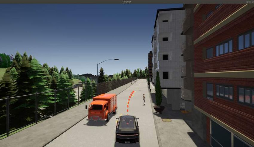
Copyright © 2020, by the author(s).
                             All rights reserved.

Permission to make digital or hard copies of all or part of this work for
personal or classroom use is granted without fee provided that copies are
not made or distributed for profit or commercial advantage and that copies
bear this notice and the full citation on the first page. To copy otherwise, to
republish, to post on servers or to redistribute to lists, requires prior specific
permission.

                               Acknowledgement

I would like to thank Professor Joseph Gonzalez for advising me through the
past 3 years. He provided incredible insight and guidance for my academic
and professional career. I would also like to thank the ERDOS Team: Ionel
Gog, Sukrit Kalra, Peter Schafhalter and Professor Ion Stoica for supporting
my research efforts.

I would like to thank Ashley for always supporting me throughout my
studies and helping me see things from different perspectives.

I would like to thank my mom, dad and brother for their unconditional and
unbounded support.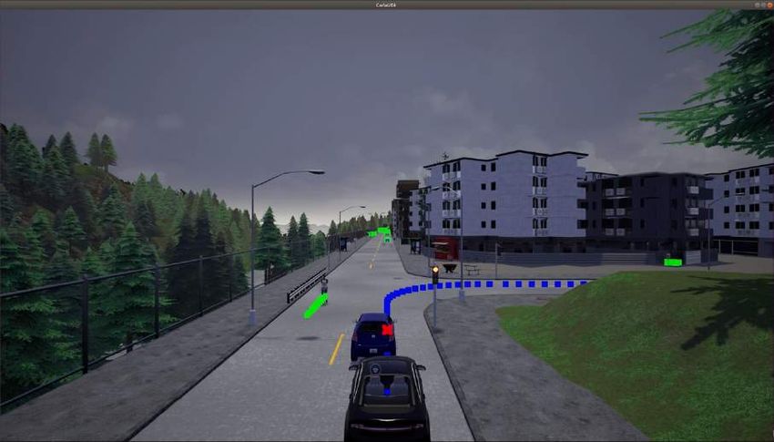
Dynamic Deadlines in Motion Planning for Autonomous Driving Systems

                                  by

                            Edward Fang

           A thesis submitted in partial satisfaction of the

                    requirements for the degree of

                         Masters of Science

                                  in

            Electrical Engineering and Computer Science

                                in the

                          Graduate Division

                                of the

                  University of California, Berkeley

                        Committee in charge:

                     Professor Joseph Gonzalez
                        Professor Ion Stoica

                             Spring 2020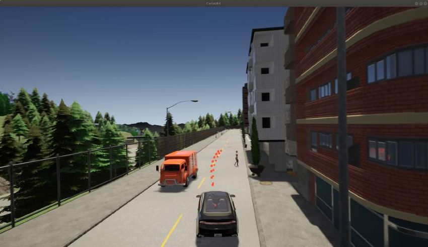
1

                                         Abstract

         Dynamic Deadlines in Motion Planning for Autonomous Driving Systems

                                             by

                                        Edward Fang

            Masters of Science in Electrical Engineering and Computer Science

                             University of California, Berkeley

                                 Professor Joseph Gonzalez

Autonomous vehicle technology is posed to increase safety and mobility while decreasing
emissions and traffic in the transportation industry. Safe, reliable and comfortable au-
tonomous vehicle technology requires the cooperation of robust driving algorithms, failsafe
hardware and real-time operating systems. While all components are important, safety-
critical motion planning algorithms are paramount as they are responsible for maneuvering
the car through complex, dynamic environments.
Motion planning is still an unsolved task in the autonomous driving realm. There are a
variety of challenges and shortcomings associated with current state of the art systems,
one primary concern being static deadline motion planning. The objective of this paper is
to explore the tradeoffs of a variety of planning algorithms in a practical, realistic driving
environment. We show how static deadlines are a limitation in current autonomous vehicle
motion planners and lay the groundwork for future work using a dynamic deadline system to
allow flexible time constraints. We propose that allowing flexible time constraints in motion
planning has significant improvements in safety, comfort and reliability over static deadline
alternatives.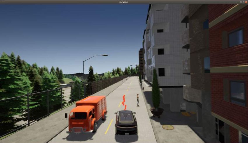
i

To my family and friends.
ii

Contents

Contents                                                                                                                                      ii

List of Figures                                                                                                                               iv

1 Introduction                                                                                                                                1

2 Overview of Autonomous Vehicle Technology                                                                                                   3
  2.1 Sensing . . . . . . . . . . . . . . . . . . . . . .                 .   .   .   .   .   .   .   .   .   .   .   .   .   .   .   .   .   4
  2.2 Perception . . . . . . . . . . . . . . . . . . . .                  .   .   .   .   .   .   .   .   .   .   .   .   .   .   .   .   .   5
  2.3 Prediction . . . . . . . . . . . . . . . . . . . .                  .   .   .   .   .   .   .   .   .   .   .   .   .   .   .   .   .   6
  2.4 Planning . . . . . . . . . . . . . . . . . . . . .                  .   .   .   .   .   .   .   .   .   .   .   .   .   .   .   .   .   8
  2.5 Control . . . . . . . . . . . . . . . . . . . . .                   .   .   .   .   .   .   .   .   .   .   .   .   .   .   .   .   .   8

3 Motion Planning Survey                                                                                                                      10
  3.1 Route Planning . . . . . . . . . . . . . . . . . .                      .   .   .   .   .   .   .   .   .   .   .   .   .   .   .   .   11
  3.2 Behavioral Planning . . . . . . . . . . . . . . .                       .   .   .   .   .   .   .   .   .   .   .   .   .   .   .   .   12
  3.3 Motion Planning . . . . . . . . . . . . . . . . .                       .   .   .   .   .   .   .   .   .   .   .   .   .   .   .   .   12
      3.3.1 Graph Search . . . . . . . . . . . . . . .                        .   .   .   .   .   .   .   .   .   .   .   .   .   .   .   .   14
      3.3.2 Incremental Search . . . . . . . . . . . .                        .   .   .   .   .   .   .   .   .   .   .   .   .   .   .   .   16
      3.3.3 Trajectory Generation . . . . . . . . . .                         .   .   .   .   .   .   .   .   .   .   .   .   .   .   .   .   18
      3.3.4 Anytime and Realtime Planning . . . . .                           .   .   .   .   .   .   .   .   .   .   .   .   .   .   .   .   20
      3.3.5 Interaction with Prediction and Control                           .   .   .   .   .   .   .   .   .   .   .   .   .   .   .   .   21

4 Motion Planning Models                                                                                                                      23
  4.1 Hybrid A* . . . . . . . . . . . . . . . . . . . . . . . . . . . . . . . . . . . . .                                                     23
  4.2 RRT* . . . . . . . . . . . . . . . . . . . . . . . . . . . . . . . . . . . . . . .                                                      27
  4.3 Frenet Optimal Trajectory . . . . . . . . . . . . . . . . . . . . . . . . . . . .                                                       30

5 Experiment Setup                                                                                                                            35
  5.1 Synchronous Carla Experiments .         .   .   .   .   .   .   .   .   .   .   .   .   .   .   .   .   .   .   .   .   .   .   .   .   36
  5.2 Asynchronous Carla Experiments          .   .   .   .   .   .   .   .   .   .   .   .   .   .   .   .   .   .   .   .   .   .   .   .   37
  5.3 Metrics . . . . . . . . . . . . . . .   .   .   .   .   .   .   .   .   .   .   .   .   .   .   .   .   .   .   .   .   .   .   .   .   39
  5.4 Scenario . . . . . . . . . . . . . .    .   .   .   .   .   .   .   .   .   .   .   .   .   .   .   .   .   .   .   .   .   .   .   .   39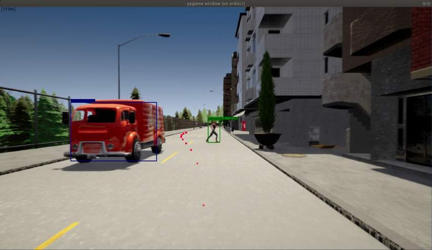
iii

6 Results                                                                                                                   41
  6.1 Runtime . . . . . . . . . . . . . . . . . . . . . .   .   .   .   .   .   .   .   .   .   .   .   .   .   .   .   .   41
  6.2 Collision Table . . . . . . . . . . . . . . . . . .   .   .   .   .   .   .   .   .   .   .   .   .   .   .   .   .   42
  6.3 Lateral and Longitudinal Metrics . . . . . . . .      .   .   .   .   .   .   .   .   .   .   .   .   .   .   .   .   45
  6.4 Lane Center Deviation and Lane Invasion Time          .   .   .   .   .   .   .   .   .   .   .   .   .   .   .   .   47
  6.5 Distance to Obstacles . . . . . . . . . . . . . . .   .   .   .   .   .   .   .   .   .   .   .   .   .   .   .   .   49
  6.6 Qualitative Results . . . . . . . . . . . . . . . .   .   .   .   .   .   .   .   .   .   .   .   .   .   .   .   .   50
  6.7 RRT* Results . . . . . . . . . . . . . . . . . . .    .   .   .   .   .   .   .   .   .   .   .   .   .   .   .   .   52
  6.8 Hybrid A* Results . . . . . . . . . . . . . . . .     .   .   .   .   .   .   .   .   .   .   .   .   .   .   .   .   57
  6.9 End-to-end with Time to Decision . . . . . . . .      .   .   .   .   .   .   .   .   .   .   .   .   .   .   .   .   60

7 Future Work                                                                                                               62

8 Conclusion                                                                                                                63

Bibliography                                                                                                                64
iv
List of Figures
2.1 A canonical example of the autonomous driving stack as a dataflow graph. . . . 3
2.2 Cruise Automation’s autonomous vehicle sensor configuration. Adapted from
General Motor’s 2018 Self-Driving Safety Report. [50] . . . . . . . . . . . . . . . 4
2.3 Object detection in Carla. Here we visualize our pipeline running end-to-end in
Carla. On screen we visualize the Faster R-CNN [57] bounding box predictions
from a first person perspective. Faster R-CNN successfully identifies the truck
and pedestrian in this scenario. This information is used by motion planning to
produce a safe trajectory between the obstacles. The trajectory is shown as red
points. . . . . . . . . . . . . . . . . . . . . . . . . . . . . . . . . . . . . . . . . . 5
2.4 Top down view of linear prediction in Carla. Cyan points are past poses and
green points are predicted future poses. Here we use the past 10 poses to predict
the next 10 poses at 10 hz. In other words, we extrapolate 1 second into the
future using a linear predictor. The scene is colored by semantic segmentation. . 7
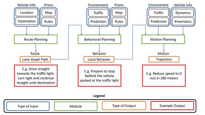
3.1 A canonical motion planning hierarchy. The rounded boxes at the top represent
various modalities of input, while the rounded boxes in the middle represent
different outputs. The boxes at the bottom serve as example outputs that feed
into downstream layers. . . . . . . . . . . . . . . . . . . . . . . . . . . . . . . . 10
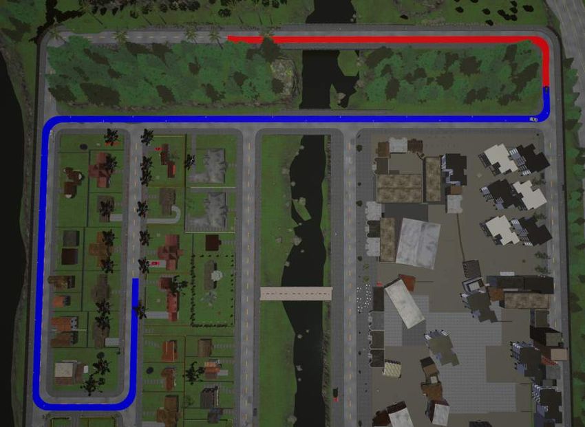
3.2 A* Route planning over the road graph in Carla. This search takes into account
the driving direction of the lane, but does not consider static or dynamic obstacles.
The nodes in the road graph are coarsely spaced waypoints on the road and the
lanes are connections between these waypoints. Here red indicates the path that
has already been covered by the ego-vehicle, while blue represents the path that
has yet to be covered. . . . . . . . . . . . . . . . . . . . . . . . . . . . . . . . . 11
3.3 A simple behavioral planner represented as a finite state machine. D denotes
driving forward along the global route. SV denotes stopping for a vehicle. SP
denotes stopping for a pedestrian. ST denotes stopping for traffic rules. O denotes
driving around an obstacle. . . . . . . . . . . . . . . . . . . . . . . . . . . . . . 12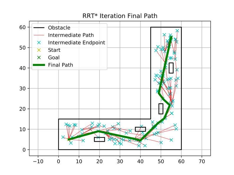
v

3.4   Planning and prediction in Carla. Here we visualize our planning and prediction
      modules in the Carla simulator. In this scenario, the ego-vehicle should follow
      the global route indicated by the blue points. Green points represent predicted
      trajectories of other agents. We note that the ego-vehicle is stopped behind a car
      at a red light. The motion planner must account for the global route, dynamic
      obstacles and traffic state to safely produce a motion plan. . . . . . . . . . . . . 13
3.5   The Probabilistic Roadmap planner. The top left figure visualizes configuration
      sampling. Pink points represent valid configurations, while black points rep-
      resent invalid configurations. The top right figure visualizes the connection of
      neighboring configurations and a validation check. The bottom figure visualizes
      the calculated path for some start, goal configuration in the PRM. These figures
      were adapted from Pieter Abbeel’s CS287 course slides [1]. . . . . . . . . . . . . 15
3.6   RRT pseudocode. RRT utilizes a tree structure to incrementally explore the
      search space. K represents the number of iterations to run RRT, xinit repre-
      sents the initial state and ∆t represents the time step discretization. RAN-
      DOM STATE returns a random state configuration from the configuration space.
      NEAREST NEIGHBOR returns the nearest neighbor of a given node. SELECT INPUT
      produces a control that connects state configurations. NEW STATE executes the
      selected control and validates for collision. Finally, the new node is added to the
      tree and corresponding edges are updated. . . . . . . . . . . . . . . . . . . . . . 18
3.7   Frenet coordinate formula. Frenet coordinates can be calculated given a set of
      points using the above formula. Frenet coordinates are represented by x, y,
      heading (θ) and curvature (κ). They are parametrized by l and d, the longitudinal
      position along a path and the lateral offset from the path. xr , yr , θr , κr represent
      the position, heading and curvature of the target path, from which we can derive
      the Frenet coordinates using the formula. . . . . . . . . . . . . . . . . . . . . . . 19
3.8   Frenet coordinate system. Above we visualize the Frenet coordinate system de-
      fined by the formula in figure 3.7. . . . . . . . . . . . . . . . . . . . . . . . . . . 20
3.9   Planning’s interaction with prediction. Here we visualize a simple scenario in
      which the ego-vehicle wishes to merge into the left lane. A naive prediction
      module may predict that the car in the left lane will continue driving forward at
      its current velocity. Prior knowledge suggests that when the ego-vehicle begins
      the merging maneuver, the vehicle in the target lane should slow down. On the
      left we visualize the state at some time t1. The blue ego-vehicle wishes to follow
      the green line, while the orange vehicle is predicted to drive straight at some
      velocity. On the right we visualize the state at some time t2 > t1. When the
      ego-vehicle begins to merge, it may predict that the vehicle in the left lane will
      slow down to accommodate the merge maneuver. . . . . . . . . . . . . . . . . . 21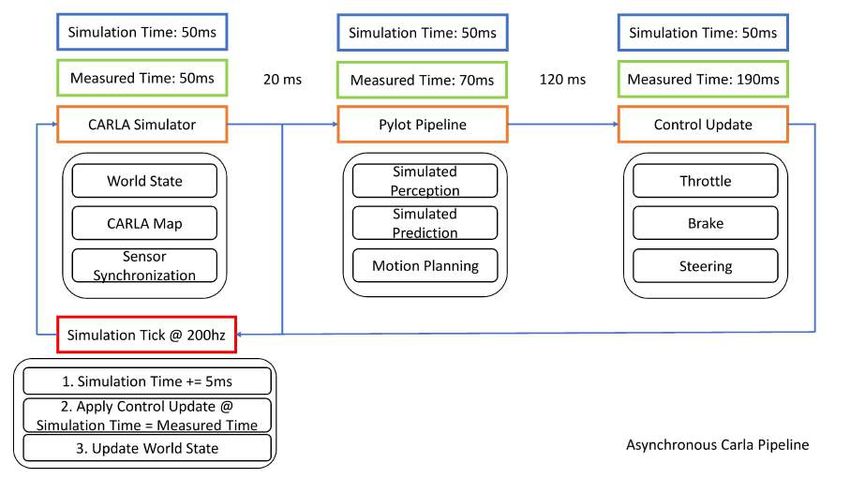
vi

4.1   Hybrid A* pseudocode. Some of the configurable variables in the code are µ
      (expansion function), completion criteria (set G), the map representation (m), δ
      (turning radius), the cost function, and the collision checking function . First,
      the search space is discretized such that each node has a continuous configuration
      range. The open set (unexplored set) is initialized with a starting position and
      associated costs. Then, until there are no more nodes to explore, we select the
      node with the minimum cost. We remove the node from the open set and add
      it to the closed set (explored set). If this node is in the goal set G, then we
      return the reconstructed path. Otherwise, we add viable neighbors to the open
      set using UPDATE. UPDATE explores new nodes by applying control inputs
      over a discretized range of possible inputs. Applying the control inputs returns a
      continuous state, which is associated with a node in the explored set. Association
      is determined by which node’s configuration range the continuous state lies in.
      If the new continuous state cannot be associated with an existing node, a new
      node with the continuous state is added to the open set. If it can be associated
      with an existing node and the new continuous state would have lower cost than
      the current associated state, we replace the current associated state. If there
      is a collision when applying the control, the node is added to the closed set.
      Otherwise, we add the neighbor to the open set. . . . . . . . . . . . . . . . . . .       24
4.2   Hybrid A* visualization. Here we visualize the Hybrid A* algorithm at vari-
      ous iterations of planning. We see how Hybrid A* search creates a branching
      pattern from nodes in the graph. The branching pattern is determined by the
      control input discretization. Here our discretization range is 15 degrees with a
      grid resolution of 0.1 m. We apply control inputs for 5 meters to explore neigh-
      boring nodes. As indicated in the legend, the cyan crosses represent intermediate
      endpoints while red lines represent paths between the endpoints. Finally, the
      minimum cost path is selected once we reach the goal. Code is available here. .           26
4.3   RRT* pseudocode. For each iteration, RRT* samples a new vertex in the con-
      figuration space. It then connects the new vertex to the neighbor that minimizes
      the path cost from x neighbor to x new. Neighbors are considered using the
      aforementioned hypersphere. Then a control input is computed and the path is
      validated for collisions. Any vertex in the vicinity of the new vertex is rewired
      if the cost to use the new vertex would be lower. Rewiring results in paths that
      are more direct than RRT paths and is necessary for optimal convergence.  q         The
                                                                                d log|T |
      radius of the N d ball is defined as a function of the size of the tree γ     |T |
                                                                                          and
      the dimensions of the search space. This is necessary to ensure that the algorithm
      asymptotically converges to an optimal path. The pseudocode is similar to RRT ,
      with the primary difference being NEIGHBORS accepting the hypersphere radius
      as a parameter and we REWIRE at the end of each iteration. SELECT INPUT
      and NEW STATE are the same as in RRT. . . . . . . . . . . . . . . . . . . . .             28
vii
4.4 RRT* visualization. Here we visualize the RRT* algorithm at different iterations
of planning. First, we note that at iteration 100, there is a path that collides with
a vehicle. This is due to the coarse discretization of the search space. Between
iteration 200 and the final graph, numerous connections are rewired for optimal
cost. This rewiring, in conjunction with the hypersphere connection process,
tends to produce very direct paths, relative to RRT. These paths are kinemati-
cally infeasible for our nonholonomic car, unless we modify the steering function.
The base steering function is just the straight line path between vertices for a
holonomic robot. Code is available here. . . . . . . . . . . . . . . . . . . . . . . 29
4.5 Frenet Optimal Trajectory costs as per [74]. vi , ai , ji are the velocity, acceleration
and jerk at time i. ci is the centripetal force measured from the center of gravity.
oj is an obstacle location. pi is a pose along the trajectory at a time i. d is the
Euclidean distance. . . . . . . . . . . . . . . . . . . . . . . . . . . . . . . . . . . 31
4.6 Frenet Optimal Trajectory costs for our implementation. vn is the final velocity
at the end of the Frenet trajectory, while vt is the target velocity. ci is the center
lane position at some time i along the target trajectory. The rest of the variables
are the same as those in figure 4.5. . . . . . . . . . . . . . . . . . . . . . . . . . 31
4.7 Frenet Optimal Trajectory visualization. Here we visualize the Frenet Optimal
Trajectory algorithms at various iterations of planning. Each of the thin red lines
is a candidate Frenet trajectory. Out of these valid candidate trajectories, the
optimal trajectory is selected with respect to our cost functions. The differences in
these trajectories reflect different discretization parameters, such as lateral offset
and target velocity. Because Frenet Optimal Trajectory does not necessarily
compute a path to the end of the trajectory, we update the world state by setting
the new configuration to the first configuration in the best candidate trajectory.
This moves the simulated vehicle forward and produces a different set of candidate
trajectories at each iteration. Code is available here. . . . . . . . . . . . . . . . 33
5.1 Synchronous Carla pipeline. Above we visualize the synchronous Carla Pipeline.
The blue boxes at the top represent simulation time, or the internal elapsed
time of the simulator. Below in green is the wall time, or the real world time.
The Carla simulator passes world state, map information and synchronized sensor
information to Pylot. Pylot runs simulated perception and prediction using Carla
internal state information and produces a control output. The control output
consists of throttle, brake and steering. Once the Carla simulator received the
control update, the simulation is ticked forward. At 20 hz, simulation time is
updated by 50 ms, the control is applied and the world state is updated for all
actors. Note that the simulation is only ticked once the entire pipeline finishes. . 37viii
5.2 Asynchronous Carla pipeline. The asynchronous Carla pipeline differs in a few
ways. First, we run at a much higher rate of 200 hz, meaning simulation time
updates by 5 ms each tick. Second, instead of wall time, we use measured time.
Finally, the simulator only applies received control at the corresponding measured
times. Measured time is the time it takes for the Pylot pipeline to produce a
control output based on when the Carla simulator outputs data. In the above
hypothetical example, it takes a total of 140 ms to produce a control output. 20
ms is due to receiving the Carla data and 120 ms is due to running the Pylot
pipeline. The time reference is 50 ms, thus the measured time is 190 ms for this
control input. When the simulation time reaches 190 ms, this control input would
be applied. . . . . . . . . . . . . . . . . . . . . . . . . . . . . . . . . . . . . . . 38
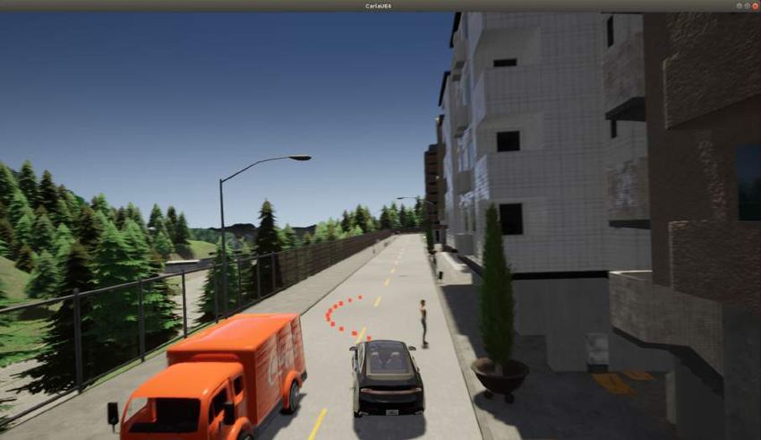
5.3 Person Behind Car scenario. The ego-vehicle must succesfully navigate between
a tight space formed by the red truck and pedestrian. . . . . . . . . . . . . . . . 40
6.1 Frenet Optimal Trajectory run-time CDF. Synchronous CDFs are on the left and
asynchronous CDFs are on the right. . . . . . . . . . . . . . . . . . . . . . . . . 42
6.2 Frenet Optimal Trajectory collision tables for synchronous cases. . . . . . . . . . 43
6.3 Frenet Optimal Trajectory collision tables for asynchronous cases. . . . . . . . . 44
6.4 Frenet Optimal Trajectory acceleration and jerk measurements for synchronous
cases. . . . . . . . . . . . . . . . . . . . . . . . . . . . . . . . . . . . . . . . . . 46
6.5 Frenet Optimal Trajectory acceleration and jerk measurements for asynchronous
cases. . . . . . . . . . . . . . . . . . . . . . . . . . . . . . . . . . . . . . . . . . 47
6.6 Frenet Optimal Trajectory lane invasion and deviation metrics for synchronous
cases. . . . . . . . . . . . . . . . . . . . . . . . . . . . . . . . . . . . . . . . . . 48
6.7 Frenet Optimal Trajectory lane invasion and deviation metrics for asynchronous
cases. . . . . . . . . . . . . . . . . . . . . . . . . . . . . . . . . . . . . . . . . . 48
6.8 Frenet Optimal Trajectory obstacle proximity metrics. Synchronous is on the
left, asynchronous is on the right. . . . . . . . . . . . . . . . . . . . . . . . . . . 49
6.9 Visualization of the Frenet Optimal Trajectory planner in the Carla pedestrian
behind car scenario. . . . . . . . . . . . . . . . . . . . . . . . . . . . . . . . . . 50
6.10 RRT* collision tables for asynchronous cases. . . . . . . . . . . . . . . . . . . . 52
6.11 RRT* run-time CDFs for asynchronous cases. . . . . . . . . . . . . . . . . . . . 53
6.12 RRT* vs. Frenet Optimal Trajectory example. The green path represents a
collision free path while the red path represents a path with collision. The red
outlines represent the collision checking function. RRT* uses a radius around
points along the path, while Frenet Optimal Trajectory uses a bounding box
collision check. Green points represent the motion planner path plan without
emergency braking. Yellow points represent the motion planner path plan with
emergency braking. The red rectangle is the truck, blue rectangle is the ego-
vehicle, and the blue circles are the pedestrian predictions. . . . . . . . . . . . . 54
6.13 RRT* lateral metrics for synchronous cases. . . . . . . . . . . . . . . . . . . . . 55
6.14 Visualization of the RRT* planner in the pedestrian behind car scenario . . . . 56ix 6.15 Hybrid A* collision tables for asynchronous cases. . . . . . . . . . . . . . . . . . 57 6.16 Hybrid A* run-time CDFs for asynchronous cases. . . . . . . . . . . . . . . . . . 58 6.17 Hybrid A* lateral metrics for synchronous cases. . . . . . . . . . . . . . . . . . . 59 6.18 Visualization of the Hybrid A* planner in the pedestrian behind car scenario. . 59
x

                                Acknowledgments
I would like to thank Professor Joseph Gonzalez for advising me through the past 3 years.
He provided incredible insight and guidance for my academic and professional career. I
would also like to thank the ERDOS Team: Ionel Gog, Sukrit Kalra, Peter Schafhalter and
Professor Ion Stoica for supporting my research efforts.

I would like to thank Professor Fernando Perez and Professor Joshua Hug for allowing me
the opportunity to teach alongside them as an undergraduate student instructor. I found
our interactions to be invaluable. To my peers, friends and fellow bears, I am indebted to
your kindness, wisdom and friendship throughout the last 5 years.

I would like to thank Ashley for always supporting me throughout my studies and help-
ing me see things from different perspectives.

I would like to thank my mom, dad and brother for their unconditional and unbounded
support.
1
Chapter 1
Introduction
Autonomous driving is the metaphorical modern day space race, in the sense that it is an
immensely challenging task that spans numerous domains. Successful self-driving systems
require innovation not only in artificial intelligence, but also in real-time operating systems,
robotic algorithms and failsafe hardware, to name a few. If self-driving matures, there
are many positive implications for society. For example, commuters who drive in dense,
urban areas waste many hours in congestion every year. Commuters in San Francisco lose
roughly 97 hours, while those in New York lose 140 hours annually [32]. Self-driving will also
benefit the environment. The transportation industry makes up 29 percent of all greenhouse
gas emissions [2]. Within transportation, over 80 percent of emissions come from vehicles
and trucks, meaning they contribute roughly 23 percent of all greenhouse gas emissions.
The number of vehicles owned has been increasing linearly over the past 2 decades [62],
inevitably contributing to emissions. Self-driving cars reduce the demand on consumer-
owned vehicles and shift vehicle transportation to a ride-sharing model that would reduce
the number of vehicles on the road, simultaneously addressing traffic and emissions concerns.
Most important, self-driving vehicles could reduce the number of fatal motor vehicle crashes.
The USA saw 34,560 fatal crashes in 2017 [70]. These crashes are due to human error, which
self-driving cars can reduce as they become mature.
Again, these are only potential benefits and only realized when autonomous technology
surpasses human level performance in terms of safety and comfort. The 34,560 fatal crashes
occurred over 3,212 billion miles, meaning human level performance is somewhere near the
order of magnitude of 1 accident per 100 million miles. Current leaders in autonomous
technology such as Waymo and Cruise have logged only 3 percent of those 100 million miles,
combined [52]. In those 3 million miles, Waymo vehicles disengaged roughly once every
13,219 miles and Cruise vehicles disengaged once per 12,221 miles. Evidently, there is a
huge gap between current state-of-the-art technology and human-level performance.
The California Department of Motorvehicles defines a disengagement as a “deactivation
of the autonomous mode when a failure of the autonomous technology is detected or when
the safe operation of the vehicle requires that the autonomous vehicle test driver disengage
the autonomous mode and take immediate manual control of the vehicle” [49]. Many of theCHAPTER 1. INTRODUCTION 2
disengagements reported by the California Department of Motor Vehicles are fundamentally
related to shortcomings of current motion planning algorithms. These disengagements range
from slight deviations from the center of the lane to potentially fatal collisions had the safety
driver not intervened. Naturally, safer motion planning will improve the true reliability of
autonomous vehicles and will be reflected in the disengagement data. While fast, real-time
planning algorithms are a must, faster does not necessarily equate to safer. It may be
advantageous to search a finer space of feasible trajectories, rather than prioritizing lower
latency. In other cases, it may be better to prioritize low latency in high-speed scenarios.
Motion planning must share its run-time with other components in the autonomous vehicle
stack and thus having a static deadline may be sub-optimal. Thus, we propose dynamic
run-time allocation for motion planning as direction towards reliable self-driving technology.
This thesis addresses the trade-offs in various types of motion planners by utilizing ER-
DOS [26] and Pylot [27] as the frameworks for developing these algorithms. We study three
different motion planning algorithms, analyze their shortcomings and strengths in practical,
realistic experiments, and propose a dynamic deadline solution to the planning problem. We
use Carla [16], a simulator designed to test self-driving vehicles, to substantiate our experi-
ments in physically realistic situations and environments. The rest of the thesis is structured
as follows: 2 presents a high-level overview of autonomous vehicle technology. 3 describes
motion planning in depth and discusses related works in motion planning. 4 details the
motion planning algorithms of interest. 5 describes the experiment setup, including imple-
mentation details, vehicle modeling, control setup and simulator configuration. 6 analyzes
the experiment results and comments on interpretability of the results. 7 discusses future
works.3 Chapter 2 Overview of Autonomous Vehicle Technology Figure 2.1: A canonical example of the autonomous driving stack as a dataflow graph. Although end-to-end approaches to self-driving exist [5], the typical autonomous driving technology stack can be decomposed into roughly 5 categories [54]: sensing, perception, prediction, planning and control. While this thesis’ focus is in planning, we still broadly describe each component as they are significant in understanding the motivation behind our
CHAPTER 2. OVERVIEW OF AUTONOMOUS VEHICLE TECHNOLOGY                                          4

method. Then, we discuss the decision-making systems used in planning and control. We
refer to our autonomous vehicle of interest as the “ego-vehicle”.

2.1      Sensing
The sensing component is responsible for ingesting streams of data regarding the driving
environment. This should contain information related to where the ego-vehicle is, where
other road users are relative to the ego-vehicle, the pose and inertial measurements of the
ego-vehicle, and so on. On-board sensors usually consist of an array of LiDARs, cameras,
GPS/INS units and radars. The data is used downstream in conjunction with prior knowl-
edge such as speed limit, traffic regulations, etc.
    Managing these sensors is difficult. All sensors need local clocks for synchronization, else
the measurements from the different sensors can be inconsistent: eg. radar measurements
and LiDAR measurements at different points in time can indicate different world states.
Time synchronization is a known research problem and while there are accepted solution
frameworks [53, 61, 20], the exact solution to a problem is highly dependent on its setup
and requirements. For example, synchronization in autonomous vehicle sensors probably
requires a higher degree of precision, as the state of the world can vary drastically given
100 ms vs 10 ms. These sensors also have different resource requirements on energy, storage
and bandwidth, further adding difficulty to the problem. While some naive solutions will
work fine for a couple of sensors, self-driving vehicles have an atypical amount and variety
of sensors to help understand the driving environment.

Figure 2.2: Cruise Automation’s autonomous vehicle sensor configuration. Adapted from
General Motor’s 2018 Self-Driving Safety Report. [50]

   For example, Cruise autonomous vehicles use 5 LIDARs, 16 cameras, and 21 radars along
with IMU, GPS, etc [50]. These streams of data operate at different rates, are variable in size,
CHAPTER 2. OVERVIEW OF AUTONOMOUS VEHICLE TECHNOLOGY 5
and produce 10s of gigabytes per second. While synchronizing and processing this amount
of data is a challenge in itself, we highlight the variability in timing as one motivation
for dynamic time allocation motion planning. Any variability in the sensing module will
generally propagate variation downstream, to perception, prediction, planning and control.
Being able to account for this variability in the other modules and in particular, motion
planning, can greatly improve safety and robustness of the autonomous vehicle.
2.2 Perception
Figure 2.3: Object detection in Carla. Here we visualize our pipeline running end-to-end in
Carla. On screen we visualize the Faster R-CNN [57] bounding box predictions from a first
person perspective. Faster R-CNN successfully identifies the truck and pedestrian in this
scenario. This information is used by motion planning to produce a safe trajectory between
the obstacles. The trajectory is shown as red points.
Perception processes data from LIDARs, cameras and radars to produce an intelligible
representation of the environment around the ego-vehicle. It typically uses a combination
of deep neural networks, heuristics and sensor fusion to produce a high definition road map.
This road map contains information such as driveable lane estimations and traffic light state
detection. Localization also takes place in the perception component, where techniques like
SLAM [18] can be applied.CHAPTER 2. OVERVIEW OF AUTONOMOUS VEHICLE TECHNOLOGY 6
For a comprehensive study of computer vision applications in autonomous vehicles, we
refer the reader to [33]. Recent advances in computer vision, namely object detection, track-
ing and activity recognition have greatly improved the onboard perception of autonomous
vehicles. Improvement in object detection is driven by region proposal methods [71] and
region-based convolutional neural networks [25]. While these models were computationally
expensive, methods such as Faster R-CNN improved run-time and turned deep neural net
approaches into viable, real-time perception algorithms. Since Faster R-CNN [57], numerous
datasets [19, 47, 22, 65, 37, 78], benchmarks [22, 47, 19] and models [33] have been developed
in the space of object detection. Tracking has also seen rapid growth, with rigorous bench-
marks such as MOT15, 16, 17 etc [43]. Current state of the art includes hybrid deep learning
and metric-based models such as DeepSORT [76] and pure deep learning approaches such
as Siamese networks [39].
These promising developments are spurred on by hardware innovations that allow for
faster, larger models with more learnable parameters. While accuracy and run-time have
improved over the years, they have generally done so in a mutually exclusive manner. Some
methods such as Faster R-CNN have been able to improve run-time while holding accuracy
constant, but usually there is a trade-off. Models with more parameters are better able to
fit the data but take longer to run. Faster models have fewer parameters, but can have
increased bias as a consequence. As shown in table 5.1 of [33], there is huge variability
across the current state of the art object detection models in terms of run-time and accuracy.
The highest accuracy model has a run-time of 3.6s/GPU while the lowest accuracy runs at
0.02s/GPU. A review [31] of speed / accuracy trade-offs in 2017 also highlights the variability
in internal model run-time, with the maximum being roughly 150 ms. These variations can
mainly be attributed to the number of objects in the scene.
In the context of self-driving, if the vehicle is moving at 10 m/s, then in 100ms the car
will have traveled 1m. At highway speeds of 25 m/s, timing is even more critical. Thus,
slight variations in perception run-time can have a significant impact on the “reaction time”
of the vehicle. It may be better to use a faster, less accurate perception model when we want
to run a higher precision motion planner, or vice-versa.
2.3 Prediction
Once the ego-vehicle understands its surroundings, it can project what the future state of
the environment could look like in the prediction component. The prediction component
foretells what other dynamic agents in the environment will do using cues from perception,
such as tracking the velocity over time and lane localization. It can also use priors of how
non-ego agents typically act under similar circumstances to utilize historical trends [58].
Other methods use a mixture of Gaussians models. For example, Waymo’s MultiPath [12]
uses a top-down scene features and a set of trajectory anchors to produce a mixture of
Gaussians model for forecasting trajectories.
The prediction component processes the state of the world constructed by perception andCHAPTER 2. OVERVIEW OF AUTONOMOUS VEHICLE TECHNOLOGY 7 Figure 2.4: Top down view of linear prediction in Carla. Cyan points are past poses and green points are predicted future poses. Here we use the past 10 poses to predict the next 10 poses at 10 hz. In other words, we extrapolate 1 second into the future using a linear predictor. The scene is colored by semantic segmentation. passes it to motion planning. It is responsible for providing accurate, reasonable information about future states of the world. It is generally accepted as an unsolved challenge as real world behaviors can be truly unpredictable. Especially in complex urban environments, there are numerous pedestrians, cyclists and vehicles to account for, not to mention other oddities like scooters, emergency vehicles and construction workers. Modelling accurate behavior for so many different types of agents is challenging. Data-driven methods such as MultiPath or R2P2 [58] can be susceptible to sampling biases, particularly where and when the data was collected. Underlying distributions can often be correlated with the time and location, so collecting sufficient amounts of data for each slice of time and location can be impractical. In extreme cases like the 6-way intersections in San Francisco, data must be actively collected in order to handle the geometry and possibilities, otherwise it would be impossible to predict
CHAPTER 2. OVERVIEW OF AUTONOMOUS VEHICLE TECHNOLOGY                                             8

future trajectories.
    In the Carla simulator, it is possible to abstract the perception problem and prediction
problem by accessing internal information such as non-ego pose and paths. Carla exposes
the world state, allowing us to query for topics such as vehicle position or traffic light state.
As this paper is concerned primarily with motion planning, our methods and experiments
abstract as much of the noise resultant from perception and prediction by utilizing the
aforementioned Carla features. In this way, we can analyze the impacts of our research as a
self-contained methodology.

2.4      Planning
The planning component must produce a safe, comfortable and feasible trajectory that
considers the present and future possible states of the surroundings. It is usually broken
down into a high-level route planner, a behavioral layer that provides abstract actions such
as “prepare to lane change left”, and low-level motion planners that produce a trajectory.
We will discuss more related work in 3.

2.5      Control
Finally, a control module actuates throttle, braking and steering to track the trajectory pro-
duced by planning. The simplest and most commonly used controller is the proportional
integral derivative (PID) controller [38], which is used to track a reference velocity in the
case of cruise control. One of the downsides is that it requires extensive tuning, as the
controller parameters are affected by different velocity, surface and steering conditions. Yet
it is effective and commercially used in many systems, including autonomous driving sys-
tems. Model-based controllers are also effective in controlling autonomous vehicles. Many
controllers utilize the kinematic bicycle model [41] to compute inputs to drive-by-wire sys-
tems [68]. Some popular controller frameworks include pure pursuit (commonly used in the
DARPA challenges [11]) and model predictive control which forward simulates an open loop
control and re-solves it for each iteration.
    Control theory is an extensive field of research and is not solely trajectory tracking. Lower
level controllers are crucial for the safety and comfort of the ride, regardless of the trajectory.
Traction control maximizes our tire friction when accelerating, braking and turning so that
the vehicle does not slip out of control. Anti-lock braking systems ensure that our braking
force is maximized and the tires do not skid. We focus on the trajectory tracking aspect of
control and discuss our control setup in section 5.
    Each of these components are required for a functional self-driving vehicle. Within each
component, there is high variability in the run-time and accuracy across different models
and internally within each model. Given this high variability, we propose that it is beneficial
to dynamically allocate run-time for different components, particularly for planning. Ac-
CHAPTER 2. OVERVIEW OF AUTONOMOUS VEHICLE TECHNOLOGY 9 counting for run-time uncertainty and adapting planning configurations on the fly can have significant impact in safety critical situations. To provide more insight, we will discuss plan- ning in depth in the following section. We show how motion planning is typically structured and cover the strengths and weaknesses of different classes of motion planners.
10

Chapter 3

Motion Planning Survey

Figure 3.1: A canonical motion planning hierarchy. The rounded boxes at the top represent
various modalities of input, while the rounded boxes in the middle represent different outputs.
The boxes at the bottom serve as example outputs that feed into downstream layers.

   At a high-level, motion planning produces a safe, comfortable and feasible trajectory
that accounts for the present and future possible states of the environment. It is usually
decomposed into 3 sub-modules: route planning, behavioral planning, and motion planning.
We will explain the challenges and solutions for each sub-module.
CHAPTER 3. MOTION PLANNING SURVEY                                                           11

3.1     Route Planning

Figure 3.2: A* Route planning over the road graph in Carla. This search takes into account
the driving direction of the lane, but does not consider static or dynamic obstacles. The nodes
in the road graph are coarsely spaced waypoints on the road and the lanes are connections
between these waypoints. Here red indicates the path that has already been covered by the
ego-vehicle, while blue represents the path that has yet to be covered.

    Route planning produces a route through a road graph given a starting and an ending
location. Edges in a road graph typically represent connections between lanes, intersections
and so on. Nodes represent points on the road and are usually coarse in resolution. For
example, vertices could only exist at intersections. Edges would then correspond to roads
connecting the intersections. The road graph representation naturally gives rise to weighted
graph search algorithms that find a minimum-cost path through the network. Popular
algorithms for route planning include A* [51], Dijkstra’s [14] and bidirectional search. These
algorithms work well for small road graphs, but are infeasible for networks with millions
CHAPTER 3. MOTION PLANNING SURVEY 12
of nodes and edges. There are numerous methods [28, 23, 6] that work around a one-off
pre-processing step that allows for much faster search later on.
3.2 Behavioral Planning
SV SP
D
ST O
Figure 3.3: A simple behavioral planner represented as a finite state machine. D denotes
driving forward along the global route. SV denotes stopping for a vehicle. SP denotes
stopping for a pedestrian. ST denotes stopping for traffic rules. O denotes driving around
an obstacle.
Behavioral planning uses the route plan and produces a high-level behavior for the vehicle
to follow. For example, if the vehicle is in the left-most lane and needs to make a right
turn, an appropriate behavior would be: prepare to change lane right. This process can be
modeled as a Markov decision process or partially observable Markov decision process (MDP
or POMDP, respectively). In the DARPA Urban Challenge, competitors used finite state
machines in conjunction with heuristics to model driving scenarios. But in the real world,
these state machines can become large and complicated due to the uncertainty of human
drivers and other traffic participants. Thus more recent work has focused on probabilistic
decision making under machine learning approaches [30, 69], model based methods [73, 77],
and MDP or POMDP models [10, 72, 9, 21, 4].
3.3 Motion Planning
For a more comprehensive and detailed overview of motion planning, we refer readers to [42,
35, 55] which serve as the basis for this discussion. We analyze the strengths and weaknesses
of a select set of motion planning algorithms which include trajectory generation, graph
search, incremental search methods, and real time planning algorithms.
Using the behavior produced by the behavioral layer, the motion planner computes a
safe, comfortable and feasible trajectory that moves the vehicle from an initial configuration
to a goal configuration. The configuration format depends on the type of motion planner:
planners that operate in the Frenet frame [75] may use a target position and lateral offsetCHAPTER 3. MOTION PLANNING SURVEY 13
Figure 3.4: Planning and prediction in Carla. Here we visualize our planning and prediction
modules in the Carla simulator. In this scenario, the ego-vehicle should follow the global
route indicated by the blue points. Green points represent predicted trajectories of other
agents. We note that the ego-vehicle is stopped behind a car at a red light. The motion
planner must account for the global route, dynamic obstacles and traffic state to safely
produce a motion plan.
along a path as the goal configuration, while a Rapidly-exploring Random Tree (RRT) [34]
planner may uses the final x, y, z position as the configuration. Regardless of the config-
uration, the motion planner must account for the road shape, the kinematic and dynamic
constraints of the vehicle and static and dynamic obstacles in the environment. Most motion
planners also optimize an objective function to eliminate uncertainty when there are multi-
ple feasible trajectories. An example of an objective function is minimizing a combination
of accumulated lateral jerk and time to destination, which are heuristics for comfort and
timeliness.
Motion planning methods can be divided into path planning methods and trajectory
planning methods. Path planning methods propose a solution that maps p(t) : [0, 1] → X ∈
C, where X is some vehicle configuration and C is the configuration space. This framework
is agnostic to time and does not enforce how a vehicle should follow the path, leaving the
responsibility to the downstream modules. Trajectory planning methods propose a solution
that maps p(t) : [0, T ] → X. This means time is explicitly accounted for in the evolution of a
motion plan. Trajectory planning methods prescribe how the vehicle configuration progressesCHAPTER 3. MOTION PLANNING SURVEY 14
with time. Under this framework, vehicle dynamics and dynamic obstacles can be directly
modeled.
Within the path planning and trajectory planning frameworks, there are numerous sub-
categories of planning algorithms. Our work focuses on analyzing Hybrid A*, RRT*, and
Frenet Optimal Trajectory. Thus in the following sections we will take a look at their cor-
responding planning subcategories, namely graph search, incremental search, and trajectory
generation, respectively. This analysis underscores potential strengths and weaknesses of
each planner and allows for further discussion in section 6, with our results.
3.3.1 Graph Search
Graph search methods represent the configuration space as a graph G = (V, E). V is a subset
of the configuration space C and E is a set of edges that connect vertices in V with a path.
Graph search methods can be further categorized as lane graph, geometric and sampling
methods.
Lane graph methods use a manually constructed graph of lanes and can be queried with
algorithms such as A* or Dijkstra’s. Geometric methods involve constructing geometric
representations of driveable regions and obstacles. Some popular geometric representations
include generalized Voronoi [66] diagrams and artificial potential fields [79]. Solutions to
geometric methods can be directly calculated from the geometric representation.
Sampling methods are generally more effective than its lane graph or geometric counter-
parts. Lane graph solutions break down when there is a dynamic agent that is unaccounted
for during the initial construction of the graph. For example, an autonomous vehicle must
be able to drive around a doubly parked car in San Francisco, but cannot do so if the road
graph had not accounted for the possibility of an obstacle at that location. Generalizing
these uncertainties leads to overly complex lane graphs and excessive manual engineering.
Geometric representations can be expensive to produce from raw sensor data. Furthermore,
the kinematic and dynamic constraints of real vehicles far exceed those provided by geo-
metric representations. For example, Voronoi diagram path planning yields discontinuous,
linear piecewise paths that are not trackable by nonholonomic vehicles. Nonholonomic sys-
tems are systems in which the number of controllable degrees of freedom are less than the
total degrees of freedom. The car is nonholonomic as we can control steering and throt-
tle, but Cartesian position (x, y) and heading (yaw) are the degrees of freedom. Sampling
methods are more popular as they can freely represent kinematic and dynamic constraints
and the configuration space. Typically, sampling based methods determine reachability of
a goal configuration using steering and collision checking steps. Steering is responsible for
producing a path from a given point A to given point B. Collision checks for collisions along
the path.
There are many types of steering functions. Random steering applies a sequence of ran-
dom controls for a period of time. Evidently, this results in suboptimal paths that are
not smooth and often far off from the goal location. Heuristic steering addresses some of
these shortcomings by applying control that progresses the vehicle towards the goal location.CHAPTER 3. MOTION PLANNING SURVEY 15
Dubin’s curve [17] and Reeds-Shepp’s curve [56] for unicycle models are exact steering proce-
dures. Exact steering procedures are usually optimal with respect to some cost function and
do not account for obstacles along the path. In particular, Dubin’s and Reeds-Shepp’s curves
are arc-length optimal under the assumption that there are no obstacles to be considered.
Thus, these exact steering procedures are generally used to connect intermediate vertices in
a graph, rather than construct a plan from the start to the goal.
Basic collision checking should take into account the vehicle geometries such as the wheel-
base length, track length, and so on. This means that pose information must be available.
Pose information can be obtained from path plans by approximating the yaw along the path.
For example, this can be done with a 2D Cubic Spline, which interpolates a series of points
using a cubic polynomial. More advanced collision checking operates in trajectory space. In
other words, it considers time as a factor in determining whether a trajectory results in a
collision. This is generally better as obstacles in the environment are dynamic, but makes
planning more dependent on a robust, accurate prediction model.
Figure 3.5: The Probabilistic Roadmap planner. The top left figure visualizes configuration
sampling. Pink points represent valid configurations, while black points represent invalid
configurations. The top right figure visualizes the connection of neighboring configurations
and a validation check. The bottom figure visualizes the calculated path for some start, goal
configuration in the PRM. These figures were adapted from Pieter Abbeel’s CS287 course
slides [1].CHAPTER 3. MOTION PLANNING SURVEY 16
Some early works in sampling based methods include the Probabilistic Roadmap (PRM)
[36] and its variants such as PRM* [34], which iteratively constructs a roadmap or an undi-
rected graph of nodes (robot configurations) and edges (feasible actions connecting configu-
rations). At a high level, PRM initializes a set of points with the start and end configuration.
Then it randomly samples points in configuration space, creating a set of valid but poten-
tially unreachable configurations. Then for each sampled configuration, nearby points are
connected if they can be reached from each other. Finally it reconstructs the plan by con-
catenating the sequence of local edge paths into a feasible path from start to goal. The edge
paths can be obtained by the aforementioned steer function and verified by the collision
function. Dijkstra’s or A* can also be used to construct these local paths. Rapidly-exploring
Random Graph (RRG) [34] is similar to PRM and PRM* in functionality and time complex-
ity, but has the added benefit of being anytime. This means an initial solution is computed
and iteratively refined until the time deadline.
Some of the challenges associated with PRM are that connecting neighboring points is
only easy for holonomic systems, ie. systems for which you can move each degree of freedom.
This typically also requires solving a boundary value problem, in which we must satisfy some
set of ordinary differential equations. Usually this is solved without considering collisions,
and then collision checking afterwards. Collision checking, although simple in concept and
not limited to just PRM, often takes the majority of time in applications [42]. There are a
variety of obstacle representations, state space discretization hyperparameters such as time
and space granularity, for example. The simplest obstacle representation is a sphere, ie.
Each obstacle has a fixed radius that must be checked for collision. There are also axis-
aligned bounding boxes, oriented bounding boxes and convex hulls, each providing a better
approximation than the previous but also more expensive to test. Finding a practical yet
safe trade-off between resolution and complexity is difficult. Furthermore, graph search
techniques suffer from poor discretization of the search space. Poor discretization can lead
to infeasibility or highly suboptimal paths. Graph search methods generate a fixed set
of nodes in the initialization, so adjusting the discretization granularity across different
iterations is not an option. High resolution discretizations are expensive to run, as the edges
in the search space increase polynomially. In our experiments, these were some of the most
significant, practical shortcomings of graph search methods. Choosing a sufficiently high
resolution discretization that could be run real time across all scenarios is challenging, and
thus motivates dynamic deadlines as a solution to this balancing problem.
We implement Hybrid A* [15], a graph search algorithm, for our experiments. Hybrid
A* associates a continuous state with each cell as well as a cost with the associated state,
and we will further discuss it in section 4.
3.3.2 Incremental Search
A key distinction between graph sampling methods and incremental search methods is that
graph sampling methods generally precompute a fixed set of nodes ahead of time, whereas
incremental search gradually builds a path by sampling the configuration space. IncrementalCHAPTER 3. MOTION PLANNING SURVEY 17
search techniques are similar to its graph sampling counterparts. It iteratively samples a
random point in the configuration space, constructs a candidate set of neighbors and connects
the new point to a neighbor using steering functions and validates using collision functions.
Again, these sampled configurations are not contained in the graph initially, whereas they
are predetermined in PRM, for example. This is one of the disadvantages of fixed graph
discretization. Search over the set of paths is limited to the initializations or primitives of
the graph discretizations. This results in solutions being infeasible or suboptimal.
Incremental search planners address this concern. They aren’t limited by the initial con-
struction of the graph and thus incremental search algorithms are generally probabilistically
complete. This means that this class of algorithms will find a solution, if one exists, given
sufficient computation time. A related term, asymptotically optimal, describes algorithms
that eventually converge to the optimal solution. One can guarantee completeness and op-
timality by repeatedly solving path planning problems over increasingly finer discretizations
of the state space. Still, incremental search techniques are unbounded in computation time.
Although a feasible solution may exist, these techniques may take asymptotically infinite
time to find it. This is a concern for real time / anytime tasks such as autonomous driving.
Another concern is the stability of random algorithms. While there are bounds and expec-
tations on the run-time and effectiveness of incremental search algorithms, the variance and
robustness of these algorithms can be an issue. Poor random seeds or slight perturbations
in obstacle locations or search space resolution can cause planners to fail. Given limited
computation time, incremental search algorithms can often fail to find even suboptimal solu-
tions, when graph search or trajectory generation methods are able to. Allocating a sufficient
amount of computation time to these planners highly upon the hyperparameter configura-
tion of the planner and the scenario the planner is operating in. Thus, dynamic allocation
may outperform static allocations as the planners are able to adapt to the driving scenario.
Many incremental search algorithms utilize tree-growing strategies in conjunction with
discretization tuning in order to get better coverage and exploration in the configuration
space. LaValle’s Rapidly-exploring Random Tree (RRT) [34] is an effective incremental
search algorithm that works well in high-dimensional settings. It builds up a tree by generat-
ing next configurations through executing random controls. Many practical implementations
will randomly attempt to connect with the end state in order to improve the run-time or
promote exploration towards the goal. In order to efficiently find approximate nearest neigh-
bors, optimizations such as KD Trees [7] or locality sensitive hashing [24] are used. These
optimizations can also be applied when representing obstacle maps. We often only need to
collision check proximal obstacles, which can be efficiently queried for using KD Trees. In
the RRT pseudo-code below, select input must solve the two point boundary value problem,
or just select the best out of a set of control sequences to find an input that moves the
robot from xrand to near. The set of control sequences can be random or some well chosen
set of primitives. Dubin’s path and Reeds-Shepp’s paths are often used as select input for
autonomous driving as they can provide arc-length optimal paths between vertices. Many
variations of RRT exist, including bi-directional RRT, resolution complete RRT (RC-RRT)
and RRT* [34], which uses heuristics to guide the exploration and tree rewiring to shortenCHAPTER 3. MOTION PLANNING SURVEY 18
Function RRT(xinit , K, ∆t)
Result: Tree T initialized at xinit
T.init(xinit )
for k = 1 to K do
xrand ← RANDOM STATE()
xnear ← NEAREST NEIGHBOR(xrand , T )
u ← SELECT INPUT(xrand , xnear )
xnew ← NEW STATE(xnear , u, ∆t)
T.add vertex(xnew )
T.add edge(xnear , xnew , u)
return T
Figure 3.6: RRT pseudocode. RRT utilizes a tree structure to incrementally explore the
search space. K represents the number of iterations to run RRT, xinit represents the initial
state and ∆t represents the time step discretization. RANDOM STATE returns a random
state configuration from the configuration space. NEAREST NEIGHBOR returns the near-
est neighbor of a given node. SELECT INPUT produces a control that connects state con-
figurations. NEW STATE executes the selected control and validates for collision. Finally,
the new node is added to the tree and corresponding edges are updated.
paths through the tree when possible. For our experiments, we implement vanilla RRT*,
which is detailed in 4.
3.3.3 Trajectory Generation
Trajectory generation methods account for kinematic, dynamic and road shape constraints
when producing a motion plan. This allows trajectory generation methods to better handle
dynamic obstacles and consider vehicle kinematics and dynamics, which is helpful when pro-
ducing controllable, feasible plans. Trajectory generation usually generates path and speed
edges separately. Paths are generated by connecting endpoints using different curvature
polynomials. After paths are generated, candidate speed profiles are built for individual
paths. To better understand the path and speed profile generation process, we describe
planning in the Frenet frame.
In the Frenet frame [75], there exists a function r(l) = [xr (l), yr (l), θr (l), κr (l)] where
l is the longitudinal offset. Let p(l, d) be a point away from the road center at the given
longitudinal offset l and d be the lateral offset away from the road center. Thus all our points
are represented as longitudinal, lateral offset pairs relative to the road center. See figure 3.7
for details. This coordinate system yields nice properties, especially for autonomous driving.
All points are represented relative to the road center, which is where we usually want ourYou can also read