EANET Research Fellowship Program 2015
←
→
Page content transcription
If your browser does not render page correctly, please read the page content below
EANET Research Fellowship Program 2015
Influence of long-range transport on air quality in
northern part of Southeast Asia during open burning season
Rungruang Janta 1), 2)*, Hiroaki Minoura 3), Somporn Chantara 1), 2), 4)
1)
Environmental Science Program, Faculty of Science, Chiang Mai University, Chiang
Mai 50200, Thailand, E-mail: rrjanta@yahoo.com
2)
Multidisciplinary Science Research Center, Faculty of Science, Chiang Mai University,
Chiang Mai 50200, Thailand
3)
Atmospheric Research Department, Asia Center for Air Pollution Research (ACAP),
1182 Sowa, Nishi-ku, Niigata-shi, 950-2144, Japan, E-mail: minoura@acap.asia
4)
Environmental Chemistry Research Laboratory, Department of Chemistry, Faculty of
Science, Chiang Mai University, Chiang Mai 50200, Thailand,
E-mail: somporn.chantara@cmu.ac.th
Abstract
Smoke haze episode occurs annually in northern part of Southeast Asia (NSEA) during the hot
dry season. Concentration of air pollutants including particulate matter with diameter less than 10 µm
(PM10), CO, NOx and O3 are 2–3 times higher than those in the rest of the year. Open burning is a major
source of air pollution in this area. This study aims to investigate an impact of long-range transport on air
quality in the NSEA during open burning season and to estimate the origin of pollutants by comparing of
PM aging at two different stations. Chiang Mai (CM) city was set as the receptor site. Based on the air
transport paths to the origin from 3-day backward trajectory during Feb–Apr for 3 years (2012–2014), air
masses were clustered into two groups for lower altitudes (500 m AGL) and three groups for higher
altitudes (1,000 m and 1,500 m AGL). Moreover, three groups of air masses from different area were also
observed from a total three attitude levels clustering. The result of air masses clustering indicated that the
major air masses through CM were transported from the southwest direction of CM and the highest level
of pollutants was originated from India region. The results revealed that the rising of air pollutant
concentration in the area was impacted from long-range transport. However, the variation of pollutant
concentration was observed in CM area. It was mainly impacted from changing of pollutant sources
(number of open burning) and metrological conditions within a day. Ratios of ions (SO42- and NO3- with
2
SO 4
K+) found in PM were used to predict their ages. The ratio in Yangon (YG) was 2 times higher
K
than that in CM. It suggested that the age of PM at CM was fresher than that in YG. Therefore, it revealed
that CM was not a receptor site receiving pollutants from YG. Characteristic of PM in CM was a mix of
aged
PM from long distance source and fresh PM emitted from local open burning, while only aged
PM from long distance source (mostly across the sea) was found in YG.
Key words: Air pollution, Backward trajectory, Biomass burning, Long-range transport, Particulate matter
aging
1. Introduction
Regarding annual smoke haze problem in Northern Thailand in the dry season, open burning
including forest fire and agricultural waste burning are the major source. This air pollution problem causes
serious degradation of economic, environment and health. Bad air quality is related to increasing of air
pollutant concentration both in form of particulate matter and gaseous pollution such as carbon monoxide
(CO), nitrogen oxide (NOx) and volatile organic compounds (VOCs). Moreover, the secondary pollutants
including ozone (O3), which is toxic to human health and vegetation, is also increasing in this period.
Concentrations of particulate matter at a size of less than 10 µm (PM10) and O3 are frequently exceeded
Thailand National Ambient Air Quality Standard at 120 μg/m3 (24 hrs average) and 200 μg/m3 (hourly
concentration) for PM10 and O3, respectively. However, the pollutants contributed in Northern Thailand
not only come from regional source but also from transportation of atmospheric pollutants over long
distance (long-range transport) (Kim Oanh and Leelasakultum, 2011). Trajectories are well known to be
good indicators of large-scale flow and can be useful for studying the potential sources of regional.
Measurement of CO along with O3 can provide evidence for the impact of anthropogenic
pollution (Lin et al., 2011 and Sikder et al., 2011). CO is one of the O3 precursors which is selected as an
indicator of long-range transport because its lifetime (1–2 months) is longer than other O3 precursors
(Suthawaree et al., 2008). Moreover, NOx which is defined as the sum of the species NO and NO2, can
also lead to O3 production. The lifetime of NO2 ranges from around 8 hrs in a typical planetary boundary
layer to a few days in the upper troposphere (Tie et al., 2001; Beirle et al., 2011; Zien et al., 2014).
Additionally, PM10 also has –3 days lifetime contribution in atmosphere (McMurry et al., 2004). Therefore,
measurement of air pollutants such as PM10, CO, O3 and NOx coupled with backward trajectory analysis
should provide information concerning effect of long-range transport on air pollution.
Large amount of organic and inorganic particles were derived from biomass burning. Potassium
(K) compounds, important inorganic particles, are commonly used as markers for biomass burning because
it does not degrade during transportation (Freney et al., 2009; Tao et al., 2016). In general, physical and
chemical properties of biomass burning particles have been changed based on the aging processes after
emission. Normally, potassium chloride (KCl) were the most abundant inorganic particle type in the young
smoke and then most of KCl particles have been converted to potassium sulfate (K2SO4) and potassium
nitrate (KNO3), through gas-particle reaction, with only minor KCl left (Li et al., 2003; Kong et al., 2015).
Gao et al. (2003) found increasing of SO42- and NO3- composition but decreasing of chloride ion (Cl-)
composition in the plum at downwind fire. Choung et al. (2015) indicated that the concentration of SO42-
and NO3- in PM at a size of less than 2.5 µm (PM2.5) increased when it is transferred to far source region.
2
Cl NO 3 SO 4
Therefore, the ratio of ions such as
,
and would help to compare the aging of PM and
K K K
indicate between near source and receptor area.
The aims of this study are to estimate the influence of long-range transport on air quality in
northern part of Southeast Asia (NSEA) during open burning season, and to investigate origins of air
pollution by comparing ratio of some ion species in PM based on backward trajectory and direction of air
mass movement. Data obtained from this research will be useful for local and governmental organizations
in term of environmental management, especially to improve air quality in the area.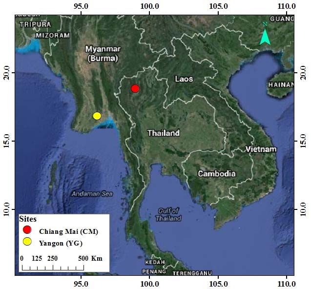
2. Method

2.1 Monitoring stations
          Base on backward trajectory, air masses arriving Chiang Mai Province during February–April
was mainly originated from the southwest direction of the province (Kim Oanh and Leelasakultum, 2011;
Chantara et al., 2012; Wiriya et al., 2013). Chiang Mai (CM), Thailand was therefore chosen as the
receptor site and Yangon (YG), Myanmar, located upwind of CM, was selected as near source sampling
site (Figure 1). Chiang Mai is the largest province in Northern part of Thailand. It is located 700 km north
of Bangkok (capital city). The province is situated between latitude 17°15′–20°06′ N and longitude
98°05′–99°21′ E at elevation of 310 meters above sea level (ASL). This area consists of valleys and hills
and forests. Mountain ranges are located in a north-south direction. North of the province is connected to
Myanmar. The province covers an area of 20,107 km2. The major land use patterns are forest (82.6 %) and
agricultural land (14.6 %) (National Statistical Office. 2012). Population density is 81.6 people/km2, in
which the highest population density is observed at Chiang Mai city (1,563 people per km2) (National
Statistical Office. 2010). Chiang Mai presents a tropical wet and dry climate which it is characterized by
the monsoon. The south-west monsoon usually arrive Thailand during the end of May–November. It
brings stream of warm moist air from the Indian Ocean causing abundant rain (rainy season). Then the
north-east monsoon starts from mid-November until mid-February and brings cool air from northern
Vietnam/China which presents cool season. The period from mid-February until the end of May is the
transition period between both monsoons and intensive thermal low therefore the hottest weather is
observed in this period. The annual average temperature is 27.0 ºC and the highest temperature is observed
in April (39.2 ºC), while the lowest is in January (11.0 ºC). The annual average humidity is 71 %. An
annual number of rainy days are 122 days with 1,075 mm the total rainfall (Northern Meteorological
Center, Thailand. 2014).
          Yangon province is the largest economic center of Myanmar. This area is located in Lower
Myanmar at the convergence of the Yangon and Bago Rivers, and is surround Andaman Sea in the south
(Yangon City Development Committee. 2016). The province is situated between latitude 17°45' - 16°12' N
and longitude 95°41'–96°49' E at elevation of 30 meters above sea level (ASL). The area within 40 km of
Yangon International Airport (17 km north of YG city hall) is covered by croplands (85 %), oceans and
seas (5 %), forests (3 %), built-up areas (3 %), and lakes and rivers (2 %). YG is the most densely
populated region in Myanmar (723 people/km2 in 2014). The climate is a tropical monsoonal character,
with three distinct seasons: a rainy season from June to October, a cooler and drier winter from November
to February, and a hot dry season from March to May. The annual mean temperature and precipitation are
27.4 oC and 2,681 mm respectively (Climatemps, 2016 and Weatherspark, 2016).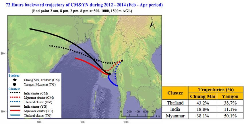
Figure 1. Map of study area.

          Figure 2 shows the location of CM observation stations comprise of Air Quality Monitoring
(AQM) station and Acid Deposition Monitoring Network in East Asia (EANET) stations. The AQM
station is located at CM city hall (18°50’N, 98°58’E), which is 5 km south of the city center. The major
land use around this station consists of community area, paddy fields and forests. EANET station
(18°46’N, 98°56’E) is located in Chiang Mai University, Mae Hia campus. It is about 5 km and 10 km in
the southwest direction of city center and AQM station, respectively. This area is surrounded by
agricultural area and forest, therefore it is classified as sub-urban area. At YG, the EANET station is
installed at Department of Meteorology and Hydrology Mayangone (16°30’N, 96°07’E). It is located in
the North of YG city hall with approximately 10 km in distance. It is surrounded by residential area, and
therefore it was characterized as urban site based on EANET criteria.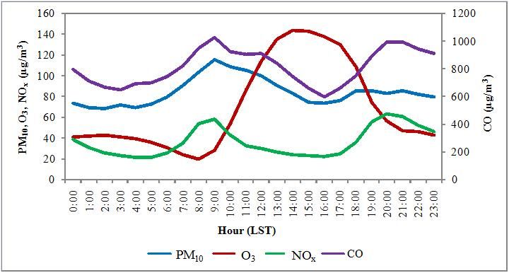
Figure 2. Location of CM station a) observation stations; b) EANET station; c) AQM
            station.

2.2 Monitoring data
2.2.1 Air pollutants
          The hourly CO, O3, NOx and PM10 concentrations from 2012 to 2014 measured at the AQM
station were obtained from Pollution Control Department (PCD), Thailand. PM10 concentration was
measured continuously using a Taper Element Oscillating Microbalance (TEOM). Ultraviolet (UV) and
chemiluminescence techniques were employed for O3 and NOx measurement, respectively. The non
dispersive infrared (NDIR) Gas Filter Correlation photometry was used for CO measurement.
          Missing data of all 3-year monitoring data used in this study was < 3 % for PM10 and O3, and
about 10 % for CO and NOx.

2.2.2 Water soluble ions
          Three year data (2012–2014) of water-soluble ions (Na+, K+, NH4+, Cl-, NO3-, SO42-) from dry
deposition analysis (particulate phase) collected from CM and YG EANET stations was provided from Asia
Center for Air Pollution Research (ACAP). The samples were collected by using the four-stage filter pack.
Each sample was collected continuously for 10days and 15days for CM and YG station, respectively. The
samples were extracted and analyzed for water-soluble ion content by using Ion Chromatograph (IC)
(EANET. 2000) (Chantara et al., 2012). Outlier data of water-soluble ions were eliminated by using
(statistic) Q-test. At 95 % confidence level 4 % (CM) and 6 % (YG) of the data were rejected.
          In order to subtract effects of sea salt ion, only non-sea-salt (nss) ions were used for nearby source
analysis. Equation (1), nss ion is calculated from subtraction of total measured ion with sea–salt (ss) ion. ss-
ion and nss-ion were calculated using equation (2) and (3), respectively. (Radojevic and Bashkin, 2003)
( EANET. 2015).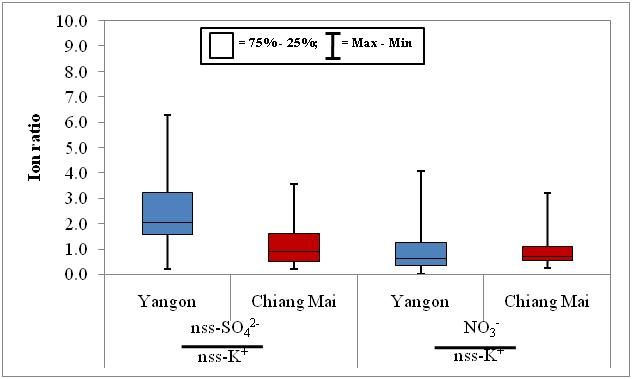
Where [nss-ionx] is non-sea-salt part of interest ion; [ionx] is total measurement of interest ion; [ss-ionx] is
X sea
sea-salt part of interest ion; [Na+] is sodium concentration;
is the ratio of interest ion and sodium ion
Na sea
in sea water. The ratios are shown in Table 1.
Table 1. Sodium and component ratio in sea water (Radojevic and Bashkin, 2003).
X sea
Ratio value by mole
Na sea
2
SO 4
0.12
Na
Cl
1.16
Na
K
0.021
Na
2.3 Air mass trajectories and air pollutants analysis
Backward trajectories of the data in the dry season (February to April) during the period of
2012–2014 were determined in order to identify the origin and transport paths of air masses and their
arrival to CM and YG. 3-day backward trajectory was normally used to determine the regional of air
pollutant distributed to Chiang Mai City from air mass movement (Somporn et al., 2012) (Soppitaporn et
al., 2013) because it could distinguish the origin of air mass for both local and long-range area in which
helpful to estimate the influence of the air mass source on pollutants contributed in the city. The origins of
air mass calculated from one day backward trajectory were observed at around the border of Thailand
(Wan et al., 2013), while 5-day backward trajectory presented very long distance of the origin (India,
Bangladesh, Myanmar and Andaman seas) which could not illustrate the local effect (Kim Oanh et al.,
2011). Therefore, 3-day backward trajectories were calculated in this study by using TrajStat-Trajectory
Statistics program version 1.2.2.6 which was developed by Yaqiang Wang in 2008 (Wang et al., 2009).
This program is using the Hybrid Single-Particle Lagrangian Integrated Trajectory (HYSPLIT) model as
an external process to calculate trajectories, and Euclidean distance clustering method as well as a
geographic information systems (GIS) technique for spatial data management, visualization and analyses.
The program was available at http://www.arl.noaa.gov/ready/hysplit4.html. The meteorological input for
the trajectory model was the GDAS (Global Data Assimilation System) and meteorological data (1° x 1°).
In this study, the backward trajectories were calculated 4 times per day (end point) at 2:00, 8:00, 14:00 and
20:00 Local Sidereal Time (LST) (19:00, 1:00, 7:00 and 13:00 UTC, respectively) for total of 268 days
during a period of 3 months (February–April) for 3 years (2012–2014). Additionally, 3 levels of an arrival
altitude were set at 500, 1000 and 1500 m AGL in order to evaluate the variance existing among trajectory
paths at different heights. Therefore, 3,216 backward trajectories per stations were calculated.Concentrations of pollutants in each calculated time were individually matched with the
clustered trajectories in order to analyze air pollutant with the categorized trajectory paths. In case of
arrival attitudes, there were assumed that pollutant concentrations in each attitude were similar in this
study.
2.4 Statistical analysis
The Spearman’s correlation among air pollutants was calculated. One way ANOVA (analysis of
variance) was used for comparison of air pollutants among the transport paths of air masses. Moreover, Q
test was employed to subtract outlier concentrations.
3. Results and discussion
3.1 Backward trajectory analysis
The selected study period (February–April) is a period of open burning in the NSEA.
Consequently smoke haze pollution is observed annually. The 3-day backward trajectories were employed
using the data of the study period (February–April in 2012–2014) at CM AQM station in order to explain
the variability and the influence of transport pathways on air pollutant contribution to air quality in CM
province. Figure 3 illustrates the clustered analysis results of 3-day backward trajectories in CM at three
arrival attitudes. Air mass patterns were classified based on their origins and directions of air masses
before arriving at the destination (CM). For reliability of clustering, number of source regions was
considered from clustering pattern which percentage of air mass contributed in all paths were greater than
10 %. Therefore, 3 clusters were classified in this study namely India (ID), Myanmar (MM) and Thailand
(TH) paths. ID path was originated from northern of India and passed over Bengal bay and Myanmar
through Chiang Mai from the southwest. MM path was initiated from India ocean or Myanmar continental
area and directly moved northeast before arriving at the site. Both ID and MM paths were represented
long-range transport of air massed in this study. Whereas TH path, was symbolized regional air mass
trajectories which came from Thailand continental area or border of Thailand and Myanmar, then directly
moved to the receptor. There were different air mass patterns with the arrival attitude. Two groups of air
masses were clustered for 500 m AGL, in which 88 % and 12 % of the trajectories were from MM and TH,
respectively (Figure 3a)). Meanwhile, three air movement paths were classified for 1000 m and 1500 m
AGL, from MM, TH and ID (Figure 3b)–3c)). The results suggested that air mass path originated from
very long distance (> 1000 km) such as ID is mainly contributed at high attitude level of air masses.a) b)
c) d)
Figure 3. Cluster of 3-day backward trajectories during February to April (2012–2014)
arrival at CM, a) 500m AGL; b) 1,000m AGL; c) 1,500m AGL; d) total 3 attitudes.
In case of the total four attitude level backward trajectories, three groups of air mass paths were
clustered (Figure 3d)). Air masses paths to CM were mainly from Western border of TH (43 %) and MM
continental area (38 %). However, all paths illustrated that air mass through CM came from southwest
direction. The results of air mass patterns were well agreed with the previous study (Chantara et al., 2012)
conducted at the same study site. They reported that the main air mass of the 3-day backward trajectories
in the dry season from 2005 to 2009 came from the southwest direction of Chiang Mai. Therefore, those
results illustrated that the air pollutants in Chiang Mai were influenced by activities along the southwest
direction through India continental area.
3.2 Air pollutants variation during 2012–2014
Concentrations of air pollutants, including PM10, O3, CO and NOx, daily rainfall and wind speed
in CM province during 2012–2014 were calculated.
3.2.1 Overview of air pollutant concentrations and some meteorological data of Chiang Mai city
Data of air pollutants, rainfall and wind speed from 2012 to 2014 were plotted (Figure 4). Rain
amount and wind speed during the study period (red boxes) were relatively lower than another period of
the year. The average wind speed in CM city was in a range of 15–30 km/hr. This value is classified as
gentle to moderate breeze in Beaufort scales. Even though increasing of wind speed was presented in April
but it was only a few days during mid to the end of month due to thunderstorm effect. Moreover, the
geography of the CM which is located in the basin surrounded by high ranges of mountain is supportingaccumulation of air pollutants in the area. The concentrations (µg/m3) of PM10, O3, CO and NOx during
February–April in 2012–2014 were 84.5 ± 43.8, 68.5 ± 16.3, 814.2 ± 453.8 and 36.6 ± 12.1, respectively.
They were 2-3 times higher than the rest of the year (Table.2).
Figure 4. Monthly concentrations of air pollutants, wind speed and rainfall of CM city in
2012–2014. Hatched period shows open burning season in the NSEA.
Table 2. Air pollutant concentrations in CM AQM station during 2012–2014.
Concentration (µg/m3)
Pollutants
PM10 O3 CO NOx
Feb–Apr Mean ± SD 84.5 ± 43.8 68.5 ± 16.3 814.2 ± 453.8 36.6 ± 12.1
(study period) Min 18.6 25.5 105.6 6.6
Max 275 112 3,241 76.5
May–Jan Mean ± SD 30.0 ± 13.9 32.4 ± 15.4 451.2 ± 294.9 21.8 ± 7.7
Min 4.7 4.4 0.0 7.4
Max 96.0 99.1 1,554 48.0
Hourly average concentrations of air pollutants from February to April 2012–2014 were plotted
(Figure 5). PM10, CO and NOx concentrations presented the same diurnal variation pattern, in which two
peaks were observed. The maximum concentrations was found around 8:00–9:00 LST, and decreasing in
the afternoon and the secondary peak was found around 20:00 LST. Due to increasing of boundary layer
height in the afternoon from increasing of temperature, the pollutants were dispersed and diluted (Zhao et
al., 2016). Whereas, the maximum O3 concentration was observed in the afternoon period because O3 is
produced during presence of solar radiation (Gao et al., 2016).Figure 5. Diurnal variation of hourly average air pollutant concentrations of CM in a period
of February–April (2012–2014).
Table 3 shows correlations among air pollutants during the study period. Significant correlations
(p < 0.01) were observed for most of all air pollutants, which were illustrated that those pollutants should
come from similar source. However, low correlations were observed between O3 and other pollutants. It
probably because O3 can be generated from various sources such as biomass burning and traffic emission
through series of physical processes and complex photochemical reactions therefore the formation
mechanism is nonlinearly related to precursors (Gao et al., 2016).
Table 3. Air pollutants correlation during February–April period 2012–2014 in CM.
Correlation
Pollutants
PM10 O3 CO
O3 0.480**
CO 0.529** 0.209**
NOx 0.750** 0.105 0.580**
Note: ** significant correlation with p < 0.01
3.2.2 Air pollutant concentrations associated with classified trajectories
According to the result from backward trajectory analysis for CM station, the variation of air
pollutants classified with air mass paths was analyzed in this section. Pollutant concentrations and the
clustered backward trajectories (3,216 trajectories) from same arrival times (end point) were matched in
order to categorize the origin of pollutants with air mass movement. Figure 6 illustrates mean
concentrations of PM10, O3, CO and NOx associated with each air mass category. Significant differences (p
< 0.05) of among clusters were found from PM10. The highest concentration was observed from ID path
(94.4 ± 55.4 µg/m3), then followed by MM path (86.8 ± 48.4 µg/m3) and TH path (78.3 ± 47.9 µg/m3).
Concentration of NOx from ID cluster (45.1 ± 30.8 µg/m3) was comparable to that from MM cluster (43.3
± 29.5 µg/m3). Nevertheless, the concentration from both clusters was higher than that from TH cluster
(39.3 ± 26.5 µg/m3). CO concentrations in descending order were ID (876 ± 603 µg/m3) > TH (849 ± 597
µg/m3) > MM (820 ± 548 µg/m3). There were no significant difference among cluster observed for CO aswell as O3. Mean concentrations of O3 for all three sites were comparable in the range of 85.9–92.2 µg/m3.
The results of this study indicated that the highest air pollutant concentration came from ID cluster, while
almost of air movement path involved in CM Province moved from TH and MM clusters.
Figure 6. Mean concentrations of air pollutants categorized by air mass pattern.
According to diurnal patterns of air pollutants within a day. Consequently arrival times of air
masses were applied to classify the pollutant concentrations in order to estimate influence of air mass paths
on the pollutants contributed in the site at different arrival times. Table 4 presents mean concentrations of
air pollutants in each arrival time and categorized air masses. Concentrations of PM10 and NOx from MM
and ID paths at 2:00 were comparable with those from regional path (TH path). Significant differences
among the paths were observed at 8:00, 14:00 and 20:00 hours. It might be because low concentrations of
long-range transport pollutants in the early morning due to low number of open burning in night time
(Reid et al., 2012). The pollutant concentrations influenced from regional source were observed in the
early morning while the daylong impacts of long-range transport were observed until evening. Impacts
from both regional and long-range sources were observed on CO concentration in CM because difference
of CO concentration was varied all the time, but no significant difference among trajectories paths was
observed. In case of O3 concentration, a significant difference among clusters was distinguished in the
afternoon. It probably because amount of O3 in this period was generated from photochemical reaction of
long-range transport ozone precursors such as NOx and CO, while local O3 or O3 generated from local
precursors were existed in another period of day.Table 4. Mean concentrations of air pollutants in each arrival time with air mass clusters.
Concentrations at various arrival altitude (µg/m3)
Arrival
Pollutants 500 m 1000 m 1500 m
time
MM TH ID MM TH ID MM TH
a a a ab b a a
PM10 2:00 69.2 62.4 87.4 64.5 63.7 73.4 63.4 66.9a
8:00 108a 70.5b 147a 100b 91.9b 118a 92.7b 99.8b
14:00 85.9a 63.3b 113a 81.1b 73.3b 93.9a 74.2b 80.2ab
20:00 85.4a 67.5b 104a 83.6b 72.4b 92.3a 78.2a 78.2a
NOx 2:00 26.4a 23.0a 29.1a 25.5ab 24.2b 27.0a 24.0a 26.5a
8:00 55.9a 42.1b 68.1a 53.8b 47.0b 62.0a 49.1b 50.2b
14:00 25.4a 20.9b 29.1a 24.9b 22.4b 26.2a 23.8a 23.9a
20:00 66.4a 42.6b 85.3a 65.5b 45.0c 72.5a 61.1ab 53.9b
O3 2:00 56.0a 64.4a 55.1a 55.3a 63.8a 56.7 a 59.2 a 54.2 a
8:00 26.6a 23.8a 21.3a 27.0a 26.3a 24.6a 28.7a 24.8a
14:00 195 a 166b 211 a 192ab 180b 205a 182b 185b
20:00 72.9a 89.0b 70.2a 71.4a 89.4a 71.7a 72.9a 81.0a
CO 2:00 646a 863b 688a 652a 717a 701a 606a 712a
8:00 982a 757a 1158a 946ab 855b 1047a 893a 910a
14:00 763a 657a 801a 754a 710a 795a 665a 801a
20:00 1015a 881a 1307a 991b 871b 1085a 934a 960a
Note: a,b,c significant difference from statistic test (p < 0.05)between cluster in the same level
3.3 Aging comparison analysis
According to the result of 3-day backward trajectory, the major air masses to CM Province
during February to April came from southwest direction (Myanmar). Therefore, aging of PM at CM and
YG stations were compared by using the ratio of water-soluble ion concentrations in PM.
3.3.1 Water-soluble ions variation
By using Table 1, concentrations of water-soluble ions (K+, Cl- and SO42-) from both stations
were listed in non-sea-salt (nss) and sea-salt (ss) fractions and presented in Table 5. The result indicated
that values of nss-Cl- were negative for both stations, which mean that it was influenced by sea salt. Thus
the concentration of nss-Cl- was excluded in this study. In case of NH4+ and NO3-, sea salt subtraction was
not necessary because of less influence from sea salt fraction.
Monthly ion concentrations (nss-K+, NH4+, NO3- and nss-SO42-) from both stations during the
period of 3 years (2012–2014) are shown in Figure 7. Those ions concentrations were significantly
correlated (p < 0.5) with of PM10 concentrations at CM-AQM station, except for NO3- from YG station.Table 5. Monthly water-soluble concentrations in 2012–2014 at CM and YG stations.
Ion concentrations (nmol/m3)
Stations Month
[ t-SO42-] [ss-SO42-] [nss-SO42-] [K+] [ss-K+] [nss-K+] [t-Cl-] [ss-Cl-] [nss-Cl-]
CM Jan 8.66 0.25 8.41 9.19 0.09 9.10 3.13 4.80 -1.67
Feb 13.93 0.55 13.39 13.55 0.20 13.35 3.58 10.63 -7.05
Mar 26.71 0.44 26.27 18.96 0.16 18.80 2.89 8.51 -5.62
Apr 9.95 0.56 9.39 11.69 0.20 11.49 2.70 10.75 -8.05
May 6.23 0.37 5.85 2.02 0.14 1.89 3.40 7.23 -3.83
Jun 5.30 0.29 5.01 1.74 0.10 1.64 4.72 5.53 -0.82
Jul 3.58 0.35 3.23 3.77 0.13 3.65 4.34 6.77 -2.43
Aug 2.00 0.25 1.75 3.30 0.09 3.21 3.10 4.81 -1.71
Sep 1.35 0.38 0.99 2.02 0.14 1.88 1.57 7.44 -5.87
Oct 19.18 0.41 18.77 6.42 0.15 6.27 1.50 7.94 -6.44
Nov 5.08 0.32 4.75 4.37 0.12 4.25 3.73 6.27 -2.54
Dec 6.61 0.28 6.33 2.85 0.10 2.74 3.71 5.49 -1.78
YG Jan 40.72 1.27 39.45 32.76 0.46 32.30 14.16 24.57 -10.41
Feb 31.70 1.06 30.63 19.26 0.39 18.87 6.67 20.59 -13.92
Mar 63.65 1.64 62.01 17.54 0.59 16.94 8.19 31.76 -23.58
Apr 20.90 0.94 19.97 10.97 0.34 10.63 5.87 18.12 -12.25
May 26.58 1.14 25.44 6.58 0.41 6.16 9.08 22.07 -13.00
Jun 3.45 0.32 3.13 3.44 0.11 3.33 9.59 6.11 3.48
Jul 18.28 2.31 15.97 3.68 0.84 2.84 17.61 44.67 -27.06
Aug 5.48 1.19 4.82 4.34 0.43 3.95 13.76 23.11 -9.35
Sep 12.82 1.05 11.81 6.65 0.38 6.27 6.16 20.31 -14.15
Oct 14.35 0.65 13.74 5.18 0.23 4.95 4.82 12.49 -7.67
Nov 21.58 0.88 20.71 18.60 0.32 18.28 7.74 16.93 -9.19
Dec 7.07 0.35 6.89 36.00 0.13 35.88 12.31 6.83 5.48
Note: total (t-); sea-salt fraction (ss-); non-sea-salt (nss-)Figure 7. Monthly ion and PM10 concentrations at CM and YG stations a) nss-SO42-;
b) NO3- ; c) nss-K+; d) NH4+.
Table 6. Ion concentrations in 2012–2014 at Chiang Mai and Yangon stations.
Concentrations (µg/m3)
Stations Feb–Apr May–Jan
nss-SO42- NO3- nss-K+ NH4+ nss-SO42- NO3- nss-K+ NH4+
Chiang Mai Mean 1.68ax 0.62ax 0.58ax 0.50ax 0.57bx 0.26bx 0.15bx 0.14bx
SD 1.83 0.61 0.58 0.55 0.82 0.21 0.17 0.19
Max 6.63 2.54 2.07 2.16 4.05 0.86 0.73 1.03
Min 0.04 0.05 0.04 0.04 0.00 0.00 0.00 0.00
n 25 25 25 25 65 65 65 65
Yangon Mean 4.03ay 0.76ax 0.66ax 0.77ax 1.49by 0.57ay 0.46ay 0.29ay
SD 4.20 0.92 0.56 0.81 1.97 0.65 0.87 0.31
Max 12.13 3.47 2.06 3.15 6.62 2.79 5.21 1.35
Min 0.10 0.00 0.02 0.00 0.00 0.00 0.00 0.00
n 16 16 16 16 49 49 49 49
Note: a,b and x,y significant difference (p < 0.05) of the same ion between study periods and stations,
respectively.
Table 6 presents ion concentrations of study period (February–April) and normal period (May–
January) of 2012–2014. Concentrations of nss-SO42-, NO3-, NH4+ and nss-K+ in µg/m3 at CM station in
study period were 1.68, 0.62, 0.50 and 0.58, respectively. Meanwhile, the concentration (µg/m3) of those
ions in YG were 4.03 (nss-SO42-), 0.76 (NO3-), 0.77 (NH4+) and 0.66 (nss-K+). The concentrations in study
period were approximately 3 times higher than those in normal period for both stations.
According to result of ion concentration comparing and correlation result between PM10 and
water-soluble ions, there were indicated that increasing of the ion concentrations during February–April
should be influenced from open burning (forest fire and agricultural burning) and relate to the rising of air
pollutant concentrations in CM.3.3.2 Ion ratio comparison analysis
Flaming and fresh smoke includes large numbers of particles containing crystals of KCl (Li et
al., 2003). Then they were converted to K2SO4 and KNO3 through gas-particle reaction during
transportation in the atmosphere (Freney et al., 2009) ( Kong et al., 2015). Therefore, the concentration
nss SO 4 NO 3
2
ratio of and between both EANET stations (CM and YG) were used in order to
nss K nss K
compare the aging of PM and indicate between near source and receptor area. Figure 8 shows the ratio of
nss SO 4
2
ions between CM and YG stations. The ratio of at YG station was around 2 times higher than
nss K
NO 3
that at CM station. Whereas, no significant difference of ratios between both stations was found.
nss K
According to instability of NO3- form in PM, it is easily interchanged with HNO3 form in aerosol due to
temperature variation (Chuang et al., 2015). Therefore, NO3- concentration of both stations should not be
related with the aging of PM. Based on the ratio values of SO42- and K+, aging of PM at YG station was
older than that at CM station.
nss SO 24 NO3
Figure 8. The ratios of and at Chiang Mai and Yangon stations during
nss K nss K
February–April in 2012–2014.
3.3.3 Air mass movement analysis
The 3-day backward trajectories were employed in order to indicate the origin of PM in YG due
to air mass movement. Total of 3,216 trajectories were classified, in which three main paths of air masses,
namely ID, MM and TH, were presented (Figure 9). Approximately 50 % of the air movement paths to
YG were started in Bengal bay and passed over only a short distance of MM continental area (MM cluster)
with a few open burning sources. Moreover, about 50% of air masses to YG, including Western of TH
(39 %) and ID continent area (11 %), were originated from neighbor countries and those air masses
transported across the sea before arrival YG site. Additionally, there was no air mass moving from middle
MM continent in the north of YG site which was one large open burning source in Southeast Asia. Those 3
paths of air masses suggested that PM in YG were mainly transported across the Bengal and Andaman Sea
and there were no additional of fresh PM originated along the air mass movement. Meanwhile, all of air
movement patterns to CM were found passing over MM continental area, the PM should be mixing ofaged PM from long distance source and fresh PM originated from open burning in the continent along the
air pathway to CM. Therefore, the aging of PM in YG was older than that in CM.
Figure 9. Cluster analysis of backward trajectories of Chiang Mai and Yangon during
February to April (2012–2014) at 3 arrival attitudes and 4 synoptic times per
day.
4. Conclusion
Open burning season (February to April) in the northern part of Southeast Asia was found to
associate with high of pollutant level and bad air quality. This period of the year 2012–2014 was selected
as the study period. Analysis of 3-day backward trajectories during study period indicated that biomass
burning in the southwest direction of Chiang Mai as well as the north of India were potential sources of
pollutants contributed in Chiang Mai Province. Moreover, long-range air movements were related to high
level of pollutants in this area. The diurnal variation of air pollutants occur mainly because of number of
biomass burning and meteorological factors changing within a day. Trajectory analysis suggested that a
part of aerosols found at Chiang Mai station come from Myanmar continent, however the degree of
particulate aging in Chiang Mai was fresher than that in Myanmar base on ions ratio comparison between
both sites. This finding was related to the geography of the area and air movement pattern to monitoring
stations. In Chiang Mai Province located in the middle of Southeast Asia continent, the PM had been
mixed from aging and fresh PM along transportation to receptor site. Whereas, Yangon located at the
Andaman coast, air masses with PM directly arrived from long distance source without additional of fresh
PM from middle of Myanmar continent area was found. Therefore, this study revealed that Chiang Mai
was not a receptor site receiving pollutants from Yangon.
Acknowledgements
Financial supports from the Network Center for the Acid Deposition Monitoring Network in
East Asia (EANET), Asia Center for Air Pollution Research (ACAP), Multidisciplinary Science Research
Center (MSRC) Faculty of Science and the Graduate School of Chiang Mai University are gratefullyacknowledged. We also thank Pollution Control Department (PCD), Thailand and Thai Meteorological
Department (TMD) for providing observation data.
References
Beirle, S., Boersma, K. F., Platt, U., Lawrence, M. G., Wagner, T., 2011. Megacity Emissions and Lifetimes
of Nitrogen Oxides Probed from Space. Science, 333: 1737-1739.
Chantara, S., Sillapapiromsuk, S., Wiriya, W., 2012. Atmospheric pollutants in Chiang Mai (Thailand) over a
five-year period (2005-2009), their possible sources and relation to air mass movement. Atmospheric
Environment, 60: 88-98.
Chuang, M. T., Fu, J. S., Lin, N. H., Lee, C. T., Gao, Y., Wang, S. H., Sheu, G. R., Hsiao, T. C., Wang, J. L.,
Yen, M. C., Lin, T. H., Thongboonchoo, N., Chem, W. C. , 2015. Simulating the transport and chemical
evolution of biomass burning pollutants originating from Southeast Asia during 7-SEAS/2010 Dongsha
experiment. Atmospheric Environment, 112: 294-305.
Climatemps, 2016. Rangoon, Yangon Climate & Temperature. http://www.yangon.climatemps.com/
EANET. 2000. Technical Document for Filter Pack Method in East Asia. Acid Deposition Monitoring
Network in East Asia (EANET), Asia Center for Air Pollution Research, Niigata, Japan.
EANET. 2015. Data report 2014, Acid Deposition Monitoring Network in East Asia (EANET), Asia Center
for Air Pollution Research, Niigata, Japan.
Freney, E. J., Martin, S. T., Buseck, P. R., 2009. Deliquescence and Efflorescence of Potassium Salts
Relevant to Biomass-Burning Aerosol Particles Aerosol. Science and Technology, 43: 799-807.
Gao, J., Zhu, B., Xiao, H., Kang, H., Hou, X., Shao, P., 2016. A case study of surface ozone source
apportionment during a high concentration episode, under frequent shifting wind conditions over the
Yangtze River Delta, China. Science of the Total Environment, 544: 853-863.
Gao, S., Hegg, D. A., Hobbs, P. V., Kirchstetter, T. W., Magi, B. I. and Sadilek, M., 2003. Water‐soluble
organic components in aerosols associated with savanna fires in southern Africa: Identification,
evolution, and distribution. Journal of Geophysical Research, 108, (D13), 8491.
Kim Oanh, N.T., and Leelasakultum, K., 2011. Analysis of meteorology and emission in haze episode
prevalence over mountain-bounded region for early warning. Science of the Total Environment, 409:
2261-2271.
Kong, S. F., Li, L., Li, X. X., Yin, Y., Chen, K., Liu, D. T., Yuan, L., Zhang, Y. J., Shan, Y. P., Ji, Y. Q.,
2015. The impacts of firework burning at the Chinese Spring Festival on air quality: insights of tracers,
source evolution and aging processes. Atmospheric Chemistry and Physics, 15: 2167-2184.
Li, J., Po´sfai, M., Hobbs, P.V., Buseck, P. R., 2003. Individual aerosol particles from biomass burning in
southern Africa: 2. Compositions and aging of inorganic particles. Journal of Geophysical Research
108, (D13), 8484.
Lin, Y. C., Lin, C. Y., Lin. P. H., Engling, G., Lan, Y.-Y., Kuo, T.-H., Hsu, W. T. and Ting, C.-C., 2011.
Observations of ozone and carbon monoxide at Mei-Feng mountain site (2269 m a.s.l.) in Central
Taiwan: Seasonal variations and influence of Asian continental outflow. Science of the Total
Environment, 409, 3033-3042.
McMurry, P. H., Shepherd, M. F., Vicker, J. S., 2004. Particulate Matter Science for Policy Makers: A
Narsto Assessment, University of Cambridge, UK.
Radojevic, M., Bashkin, V. N., 2003. Practical Environmental Analysis (2nd Ed), the Royal Society of
Chemistry, UK.Reid, J. S., Xian, P., Hyer, E. J., Flatau, M. K., Ramirez, E. M., Turk, F. J., Sampson, C. R., Zhang, C.,
Fukada, E. M., Maloney, E. D., 2012. Multi-scale meteorological conceptual analysis of observed active
fire hotspot activity and smoke optical depth in the Maritime Continent. Atmospheric Chemistry and
Physics, 12: 2117-2147.
Sikder, H. A., Suthawaree, J., Kato, S., Kajii, Y., 2011. Surface ozone and carbon monoxide levels observed
at Oki, Japan: Regional air pollution trends in East Asia. Journal of Environmental Management, 92:
953-959.
Sillapapiromsuk, S., Sato, K., Chantara, S., 2013. Assessment of Long-Range Transport Contribution on
Haze Episode in Northern Thailand, year 2007. EANET Science Bulletin, 3: 25-40.
Suthawaree, J., Kato, S., Takami, A., Kadena, H., Toguchi, M., Yogi, K., Hatakeyama, S., Kajii, Y., 2008.
Observation of ozone and carbon monoxide at Cape Hedo, Japan: Seasonal variation and influence of
long-range transport. Atmospheric Environment, 42: 2971-2981.
Tao, J., Zhang, L., Wu, Y., Zhang, Z., Zhang, X., Tang, Y., Cao, J., Zhang, Y., 2016. Uncertainty assessment
of source attribution of PM2.5 and its water-soluble organic carbon content using different biomass
burning tracers in positive matrix factorization analysis — a case study in Beijing, China. Science of the
Total Environment, 243 (A): 326-335.
Tie, X., Zhang, R., Brasseur, G., Emmons, L., Lei, W., 2001. Effects of lightning on reactive nitrogen and
nitrogen reservoir species in the troposphere. Journal of Geophysical Research, 106: 3167-3178.
Wang, Y.Q., Zhang, X.Y., Draxler R. R., 2009. TrajStat: GIS-based software that uses various trajectory
statistical analysis methods to identify potential sources from long-term air pollution measurement data.
Environmental Modelling& Software, 24: 938-939.
Weatherspark, 2015. Average Weather for Yangon (Rangoon), Myanmar (Burma),
https://weatherspark.com/averages/33996/Yangon-Rangoon-Yangon-Division-Myanmar-Burma-
Wiriya, W., Prapamontol, T., Chantara, S., 2013. PM10-bound polycyclic aromatic hydrocarbons in Chiang
Mai (Thailand): Seasonal variations, source identification, health risk assessment and their relationship
to air-mass movement. Atmospheric Research, 124: 109-122.
Yangon City Development Committee. 2016. http://www.ycdc.gov.mm
Zhao, S., Yu,Y., Yin, D., He, J., Liu, N., Qu, J., Xiao, J., 2016. Annual and diurnal variations of gaseous and
particulate pollutants in 31provincial capital cities based on in situ air quality monitoring data from
China National Environmental Monitoring Center. Environment International, 86: 92-106.
Zien, A. W., Richter, A., Hilboll, A., Blechschmidt, A.-M., Burrows, J. P., 2014. Systematic analysis of
tropospheric NO2 long-range transport events detected in GOME-2 satellite data. Atmospheric
Chemistry and Physics, 14: 7367-7396.You can also read