Economic feasibility of wood-based structures-Improving urban carbon neutrality strategies - IOPscience
←
→
Page content transcription
If your browser does not render page correctly, please read the page content below
LETTER • OPEN ACCESS

Economic feasibility of wood-based structures—Improving urban carbon
neutrality strategies
To cite this article: Ilmari Talvitie et al 2021 Environ. Res.: Infrastruct. Sustain. 1 011002

View the article online for updates and enhancements.

                                 This content was downloaded from IP address 46.4.80.155 on 03/08/2021 at 11:45
Environ. Res.: Infrastruct. Sustain. 1 (2021) 011002 https://doi.org/10.1088/2634-4505/abfe05
LETTER
Economic feasibility of wood-based structures—Improving
O P E N AC C E S S
urban carbon neutrality strategies
R E C E IVE D
17 March 2021
Ilmari Talvitie ∗ , Jussi Vimpari and Seppo Junnila
R E VISE D
28 April 2021
Aalto University School of Engineering, Department of Built Environment, Finland
∗
Author to whom any correspondence should be addressed
AC C E PTE D FOR PUBL IC ATION
4 May 2021 E-mail: ilmari.talvitie@aalto.fi
PUBL ISHE D Keywords: wood-based structures, carbon neutrality, housing economics, economic feasibility
24 June 2021
Original content from
this work may be used Abstract
under the terms of the Countries and cities alike have set carbon neutrality goals for the near future. Urban areas are
Creative Commons
Attribution 4.0 licence. experiencing an increased demand for new housing developments, and buildings are responsible
Any further distribution for one third of all greenhouse gas emissions. The relative share of construction emissions is
of this work must
maintain attribution to increasing as energy production is de-carbonizing. Wooden structures have showcased potential in
the author(s) and the substantially decreasing these emissions. However, for the construction industry to utilize
title of the work, journal
citation and DOI. environmentally friendly products, the cost efficiency needs to be determined. Prior research does
not present conclusive results regarding the construction costs or value of wooden buildings. This
study aims to determine the economic feasibility of wood-based structures in housing.
We approach this by estimating the effect of wood on Finnish dwelling prices through hedonic
regression analyses. Dwelling prices are analysed with transaction data from the Helsinki
metropolitan area. It is provided by the Central Federation of Finnish Real Estate Agencies. The
data represents occurred transactions between 1999 and 2018. The study discovers that a wooden
structure has a positive price effect in the Helsinki metropolitan region suggesting an economically
feasible opportunity to create low carbon urban housing. In the city of Helsinki, the effect is
statistically significant (+8.85%) whereas no significance is found in either Espoo or Vantaa. The
results suggest that in Helsinki, a direct financial benefit exists for both the city and private
developers. For other cities, the study encourages the increase of consumption of wood due to its
environmental properties. The study implies that wooden construction is an economically feasible
solution in mitigating climate change. As this may provoke an increased demand for wood in
construction, further research should be conducted to analyse its effects on the economy and the
environment.
1. Introduction
Over half of the global population is currently living in urban areas and continuing urbanization increases
demand for new residential developments. This growth is embodied by an amplified amount of multi-storey
construction as land in urban areas is not abundant. At the same time, the building and construction sector is
accountable for nearly 40% of global greenhouse CO2 emissions (IEA 2020). Construction accounts for over
a quarter of these emissions, but for new developments, a building’s construction phase can account for over
half of its lifecycle emissions (Säynäjoki et al 2012). As buildings’ operational phase emissions decrease with a
cleaner energy system, the importance of decreasing construction-related emissions grows.
An increasing amount of cities across the globe are setting ambitious carbon neutrality goals for the near
future, e.g. Copenhagen to 2025 and Glasgow to 2030 (CNCA 2021). It has been pointed out that these goals
are not attainable if construction emissions are not decreased significantly (Säynäjoki et al 2012). One of the
key challenges is to use more environmentally friendly materials as main building structures. Recently, Amiri
et al (2020) presented that wood-based structures could decrease construction related emissions by half. Addi-
tionally, it has been presented that cities could become carbon sinks as wood can store carbon (Buchanan and
Levine 1999 and Amiri et al 2020).
© 2021 The Author(s). Published by IOP Publishing LtdEnviron. Res.: Infrastruct. Sustain. 1 (2021) 011002
Given these promising abilities, why is wood not used more extensively in construction? A plethora of
research has been conducted globally about the barriers that hinder the use of wood in construction (Nykänen
et al 2017, Thomas and Ding 2018, Jones et al 2016 and Djokoto et al 2014). The barriers range from a lack
of knowledge and expertise (Nykänen et al 2017) to the conservative path-dependency of the construction
industry (Jones et al 2016). A major barrier is the perception of higher construction costs (Nykänen et al 2017,
Jones et al 2016, Thomas and Ding 2018 and Djokoto et al 2014). This study approaches the latter barrier, since
research implies that for wood to be a feasible solution in mitigating climate change, it must be cost-competitive
(Petersen and Solberg 2005).
Prior research is not conclusive as to whether or not wood construction is more expensive. Some argue costs
to be lower (e.g. Hossaini et al 2015 and švajlenka et al 2017) and others higher for wood (e.g. Cazemier 2017).
Koppelhuber et al (2017) imply that costs are case-dependent. Jones et al (2016) presents that higher material
costs of wood-based products can be offset through faster construction speed. Wood-based construction is
generally recognized to be significantly faster than traditional non-wooden construction (Kremer and Ritchie
2018, Richie and Stephan 2018 and Mäkimattila 2019). The faster construction times can generate a better
return on investment for developers (Cazemier 2017) and decrease negative externalities, such as noise and
dust, from construction (švajlenka et al 2017). Interestingly, research that has found wooden construction to
be more expensive now, believe it to become less expensive in the future (Jones et al 2016). Cazemier (2017)
bases this argument on increased knowledge and progression of construction methods in the future. However,
Mäkimattila (2019) argues that wood-based construction will become relatively more expensive in Finland
due to increasingly cheaper concrete elements.
Literature presents no definitive results on the economic feasibility of wooden structures through con-
struction costs. Moreover, to the best of our knowledge, there is no prior research on wooden structure’s effect
on residential dwelling prices. This paper aims to shed light in this research gap by examining the economic
feasibility of wooden structures in Finland with the following research question:
RQ: Do wooden apartments have a price premium in the Helsinki metropolitan area?
In this study, we present how wood affects apartment building dwelling prices in the Helsinki metropolitan
area (HMA) through hedonic regression analyses. The regression analyses enable the research to single out the
effect of all explanatory variables used. The interest in this study is set on the building material.
2. Methodology
2.1. Research approach
Bostic et al (2007) describe a dwelling as a bundled good, where its price is determined by a variety of inter-
twined housing characteristics, such as size, age and location. They further suggest that no single feature
can determine a dwelling’s price. Therefore, a sufficient amount of features should be used when estimating
dwelling prices.
Prior and similar research use a hedonic regression analysis as a tool in estimating dwelling prices (Rosen
1974 and Fuerst et al 2016). A hedonic regression analysis estimates dwelling prices based on used data and vari-
ables. Hedonic regression analysis assigns each variable a ß-value that defines the effect size on the dwelling’s
estimated price. The hedonic regression model used in this paper is adapted from Fuerst et al (2016):
ln(P(i, j)) = β0 + β1 ∗ W(i, j) + β2 ∗ X(i, j) + y(i, j) + e(i, j) (1)
where,
P(i, j) = price of the ith dwelling in jth neighbourhood
W(i, j) = building material (wood)
X(i, j) = vector for housing and neighbourhood characteristics
y(i, j) = postal codes
e(i, j) = error term of the regression.
Equation (1) presents the most appropriate model found for this study to predict dwelling prices in the
HMA. The dependent variable (P) is the natural logarithm of the price of a dwelling. This study attempts
to predict the price through the building material, housing and neighbourhood characteristics and the postal
codes of neighbourhoods. ß0 represents the equation constant, ß1 conveys the coefficient of the building mate-
rial wood, and ß2 is a vector of housing and neighbourhood coefficients. These vectors in the regression model
are estimated via a simple ordinary least squared regression. The regression is clustered by postal codes that
control the model’s error term. This method is used by Fuerst et al (2016) who further express that the clus-
tering of postcodes may lead to incorrect assumptions of the residuals being identically and independently
distributed. They imply it is a result of dwelling transactions occurring in the same location in different occa-
sions. Regardless, when clustering error terms the regression, estimates are unbiased, but the standard errors
2Environ. Res.: Infrastruct. Sustain. 1 (2021) 011002
may be incorrect (Fuerst et al 2016). However, Rogers (1993) indicates that it is normal for features to correlate
only within the areas in an unobserved manner.
Regression is used to estimate dwelling prices for each city separately in the HMA as well as the entire region
as one. The regression analyses follow the stepwise-method (Mellin 2006). The analyses are conducted on a
95%-confidence interval. Since the regression analysis follows the stepwise method, all variables in the final
regression are statistically significant on a 95%-confidence interval. Additionally, it is good to note a rule of
thumb for regression analyses in general. If the variation inflation factor (VIF) is above 10, the regression expe-
riences problems of multicollinearity. These problems can mark a regression coefficient’s effect as unreliable.
Therefore, the study opts to exclude variables that lead to high multicollinearity.
2.2. Dwelling transaction data
This research utilizes data of occurred dwelling transactions in the HMA during 1999– 2018. HMA is the largest
metropolitan area (1.18 million population) in Finland comprising the capital city of Helsinki as well as two
of its neighbouring cities Espoo and Vantaa. The data is provided by the Central Federation of Finnish Real
Estate Agencies (KVKL 2020).
The dwelling transaction data is allocated to three separate datasets based on the building’s construction
year. Dwellings constructed between (1) 1990 and 2020, (2) 2000–2020, and (3) 2010–2020. The division is
conducted since wooden construction is currently undergoing a strong period of growth. Therefore, based on
this trend the study attempts to uncover whether the market is experiencing changes in newer dwellings. The
following descriptions and results will detail the data for the complete data period of 1990–2020.
Furthermore, the original study analyses the effect of wood on the prices of three different dwelling types;
(1) apartment building, (2) semi-detached, and (3) detached dwellings. However, for the purposes of this
paper, results of only apartment building dwellings are presented. The reason is due the increasing demand for
land in cities which has directed increasing amounts of multi-storey developments to urban areas. Therefore,
the results regarding semi-detached and detached dwellings are not of interest in this paper.
In addition to the location, construction year and building type, the dwelling transaction data conveys
a multitude of housing characteristics that have been used in prior hedonic analysis research (Sirmans et al
2006). Table 1 presents the descriptive statistics of these variables. The data is further processed by dividing
the transaction price by the dwelling’s size. This provides a standardized price variable, price per square meter,
to assist in detecting outlying observations. Null values and observations with a distance over 3.29 standard
deviation of price per square meter are removed as outliers.
The dwelling transaction data is supplemented by a wide range of neighbourhood characteristics. This
data is provided by Statistics Finland (2020). The neighbourhood characteristics data portrays socio-economic
features on a 250 × 250 m grid in Finland. The grid data used in this study comprises socio-economic infor-
mation from the following years: 2000, 2005, 2010–2016, and 2018. These datasets are joined to the dwelling
transaction data based on the transaction year of a dwelling to gain a more accurate depiction of the sold
dwelling. The grid data provides detailed information regarding a neighbourhood’s locational attributes, such
as average income level, unemployment rate, and the number of families with children in a neighbourhood
(table 1). Fuerst et al (2016) detail that neighbourhoods globally can be very small and may vary distinctly from
each other. For example, ‘good’ and ‘bad’ areas may be in close proximity to each other. These features affect
the attractiveness of a dwelling. Thus, neighbourhood characteristics in addition to housing characteristics
strengthen the estimation of dwelling prices.
Finally, the research supplements a variable detailing a dwelling’s Euclidean distance to the city centre
of Helsinki. The variable addition is based on a monocentric city model which dictates that dwelling prices
decrease the further away they are from a city centre (Brueckner 2011). The distance to the centre area is there-
fore a crucial element in determining dwelling prices. The variable is calculated in QGIS with the distance to
the nearest HUB-tool. The HUB, i.e. centre, was defined as the main railway station of Helsinki. The regression
analysis is further supplemented with the variable ‘Sold during or after 2011’. It is selected since regulations for
wooden multi-storey buildings changed during 2011 (Nykänen et al 2017 and Ruuska and Häkkinen 2016)
and the study considers that it may affect consumer attitudes.
Table 1 presents all central variables used in the regression model. The variables are separated by housing
characteristics and neighbourhood characteristics. The dependent variable price is not presented since price
per square meter provides a more indicative view on the mean price. The figure showcases all observations’
descriptive statistics in the HMA in the first column, and all the wooden observations’ in the second. These
columns are followed by the descriptive statistics of Helsinki, Espoo and Vantaa separately. It is important to
understand how wooden dwellings are detailed in the data. The following section will elaborate on what a
wooden dwelling is and how it is described in the data.
3Environ. Res.: Infrastruct. Sustain. 1 (2021) 011002
Table 1. Summary statistics of regression variables.
Summary statistics HMA all observations HMA wooden observations Helsinki all Helsinki wood Espoo all Espoo wood Vantaa all Vantaa wood
Mean Std.dev Mean Std.dev Mean Std.dev Mean Std.dev Mean Std.dev Mean Std.dev Mean Std.dev Mean Std.dev
Housing characteristics
Price (€/m2 ) 3,988.40 1,419.87 3,718.56 932.11 4,271.92 1,604.94 3,730.37 989.22 3,800.47 1,139.35 3,442.91 740.99 3,489.81 990.37 3,844.41 954.48
Size (m2 ) 64.16 22.26 54.89 16.74 67.35 23.93 58.00 20.13 63.33 19.50 57.94 13.79 56.85 19.08 51.59 15.20
Built year 2,005.20 7.42 2,006.92 9.28 2,005.00 7.34 2,006.08 7.82 2,004.68 6.76 2,004.39 8.52 2,006.44 8.27 2,008.63 10.08
1 0.09 0.28 0.14 0.35 0.07 0.26 0.18 0.38 0.07 0.25 0.08 0.28 0.15 0.36 0.15 0.35
2 0.46 0.50 0.46 0.50 0.45 0.50 0.43 0.50 0.47 0.50 0.44 0.50 0.47 0.50 0.49 0.50
Rooms 3 0.31 0.46 0.30 0.46 0.31 0.46 0.28 0.45 0.34 0.47 0.39 0.49 0.28 0.45 0.27 0.45
Excellent 0.01 0.09 0.04 0.18 0.01 0.10 — — 0.01 0.08 0.01 0.12 0.01 0.11 0.07 0.25
Good 0.80 0.40 0.67 0.47 0.79 0.41 0.68 0.47 0.85 0.35 0.81 0.40 0.77 0.42 0.59 0.49
New 0.07 0.26 0.21 0.40 0.07 0.25 0.25 0.43 0.03 0.18 0.12 0.32 0.13 0.33 0.22 0.42
Decent 0.07 0.25 0.08 0.26 0.08 0.27 0.06 0.23 0.05 0.21 0.04 0.20 0.05 0.22 0.10 0.30
4
Poor 0.00 0.03 — — 0.00 0.03 — — 0.00 0.02 — — 0.00 0.04 — —
Condition Other 0.05 0.22 0.02 0.13 0.05 0.22 0.01 0.11 0.06 0.24 0.02 0.14 0.03 0.18 0.02 0.14
New development (dummy) 0.42 0.49 0.33 0.47 0.43 0.49 0.33 0.47 0.39 0.49 0.15 0.36 0.44 0.50 0.42 0.49
Elevator (dummy) 0.76 0.43 0.13 0.34 0.78 0.41 0.32 0.47 0.75 0.43 0.14 0.35 0.72 0.45 0.02 0.13
Owned 0.76 0.43 0.64 0.48 0.62 0.49 0.24 0.43 0.95 0.22 0.65 0.48 0.87 0.34 0.87 0.34
Rented 0.23 0.42 0.35 0.48 0.37 0.48 0.73 0.45 0.03 0.18 0.34 0.47 0.13 0.34 0.13 0.33
Lot ownership Other 0.01 0.10 0.01 0.12 0.01 0.10 0.03 0.17 0.01 0.12 0.01 0.12 0.01 0.07 0.01 0.08
Distance to CBD (km) 9.71 4.62 13.74 4.05 6.83 3.60 9.17 2.13 12.00 3.07 15.07 2.81 14.24 3.14 15.78 3.19
Sold during or after 2011 0.56 0.50 0.76 0.43 0.54 0.50 0.62 0.49 0.53 0.50 0.71 0.46 0.64 0.48 0.87 0.33
Neighbourhood characteristics
Population 517.41 336.68 315.65 222.81 620.57 373.45 507.34 264.40 422.73 262.96 287.83 118.05 370.52 203.51 216.34 152.56
Mean income per capita (€/year) 25,505.54 8,625.90 26,929.65 7,074.36 26,206.23 10,325.49 23,331.94 4,237.34 25,811.18 7,087.54 29,949.17 7,251.78 23,263.13 3,878.38 27,590.66 7,450.19
Number of buildings 12.85 8.46 23.84 12.56 12.48 8.01 20.17 10.18 13.24 8.41 26.77 15.10 13.33 9.56 24.59 12.02
Mean dwelling size (m2 ) 64.37 12.43 74.31 16.53 64.31 12.10 67.86 11.75 66.04 14.24 74.18 16.96 62.34 10.26 78.17 17.55
Share of university education 0.25 0.14 0.38 0.15 0.25 0.14 0.36 0.12 0.25 0.15 0.46 0.18 0.25 0.11 0.34 0.13
Share of families with children 0.17 0.10 0.17 0.16 0.17 0.09 0.14 0.10 0.17 0.11 0.16 0.17 0.16 0.12 0.20 0.17
Share of home-owners 0.11 0.18 0.20 0.30 0.11 0.17 0.09 0.14 0.10 0.17 0.23 0.32 0.13 0.20 0.25 0.34
Umemployment rate 0.40 0.29 0.36 0.35 0.40 0.28 0.30 0.25 0.43 0.30 0.41 0.36 0.36 0.30 0.38 0.39
Pensioner share 0.34 0.15 0.27 0.19 0.35 0.15 0.30 0.17 0.38 0.15 0.32 0.23 0.26 0.12 0.23 0.17Environ. Res.: Infrastruct. Sustain. 1 (2021) 011002
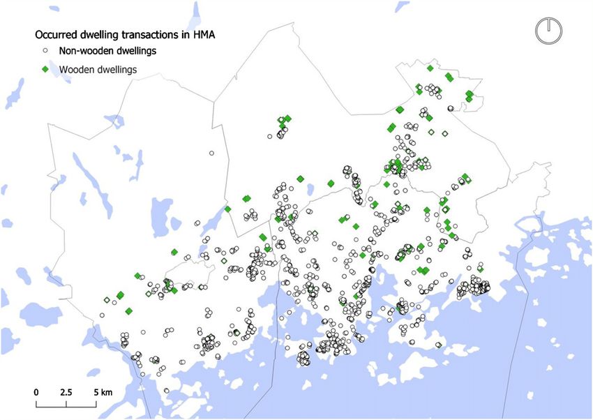
Figure 1. Occurred apartment building dwelling transactions in the HMA.
2.3. Wooden structures in the data
A wooden dwelling in this study is defined as a flat located in a building which is fully constructed of wood or
contains a wooden frame, e.g. buildings with a wooden frame but a brick facade are considered as a wooden
building in this study. Unfortunately, in most cases the data descriptions only detail the main building material
which can lead to incorrect material categorisations for dwellings. The data was processed carefully to avoid
this. The dwelling transaction data is presented in the Finnish language, thus, the following descriptions are
translated into English by the authors. These material descriptions convey the definitions of wooden apartment
building dwellings presented in the data;
(a) ‘Wood’ (obs. count 404)
(b) ‘Wood’ (obs. count 208)
(c) ‘CLT-frame with wooden façade’ (obs. count 11).
Wood’s share of buildings is only 2.23%. The city of Helsinki contains 177 of these observations, the city of
Espoo 145, and the city of Vantaa 301. Figure 1 presents a map that conveys the occurred transactions of apart-
ment building dwellings, which have been constructed between 1990 and 2020 and sold between 1999–2018.
The green diamonds present wood and the white circles non-wooden observations. It is good to note that
the observations are located in multi-storey developments, therefore, each mark in the figure can represent
multiple observations.
3. Results
Table 2 presents regression results based on the model and methods showcased in section 2.1. The table details
the effect of wood, the explanatory power, sample size, and variable-groups used in each of the regression
analyses. The brackets following the variable group ‘postal codes’ indicates the amount of clusters used in the
regression analyses. Each regression uses the same base model, however, the resulting regression models differ
from each other due to the stepwise-method. The statistically significant variables are presented in table 3.
In table 2, the results for the HMA present that a wooden structure has a positive effect (ß-value = 0.017)
on dwelling prices in the entire region. However, based on a 95% confidence interval the effects is not statisti-
cally significant (p = 0.498). The explanatory power, adjusted R-squared, value is nearly 91%. Therefore, the
study does not consider adding additional variables. The regression analysis does not indicate any problems of
multicollinearity (VIF < 10).
To study the HMA in more detail, additional regression analyses were conducted for each city separately.
The reason behind the additional analyses is due to each city having their own urban development and housing
5Environ. Res.: Infrastruct. Sustain. 1 (2021) 011002
Table 2. Regression estimates for transaction prices. ∗ p-value < 0.05, ∗∗ p-value < 0.01, ∗∗∗ p-value < 0.001.
(a)–(c) are presented in table 1. [Brackets] convey the amount of postal codes.
(1) HMA (2) Helsinki (3) Espoo (4) Vantaa
Effect of wood 0.017 0.085∗∗∗ 0.029 −0.011
Std. err. [0.025] [0.020] [0.037] [0.022]
R-squared 0.907 0.91 0.891 0.876
Adj R-squared 0.906 0.909 0.89 0.875
Sample size 27 954 14 867 7422 5665
Wooden observations 623 177 145 301
% of wooden obs. 2.23 % 1.19 % 1.95 % 5.31 %
Postal codes Yes [137] Yes [79] Yes [33] Yes [25]
(a) Housing characteristics Yes Yes Yes Yes
(b) Neighbourhood characteristics Yes Yes Yes Yes
(c) Distance to CBD Yes Yes Yes No
Table 3. Statistically significant variables.
(1) HMA (2) Helsinki (3) Espoo (4) Vantaa
Housing characteristics
Size (log)
Age (log)
Rooms 1
2
3
Condition Excellent
Good (control variable) — — — —
New
Decent
Poor
Other
New development (dummy)
Elevator (dummy)
Lot ownership Owned
Rented (control variable) — — — —
Other
Distance to CBD (log)
Sold during or after 2011
Neighbourhood characteristics
Population (log)
Mean income per capita (log)
Number of buildings (log)
Mean dwelling size (log)
Share of university education
Share of families with children
Share of home-owners
Unemployment rate
Pensioner share
programmes. Therefore, individual analyses provide each city with detailed results in regard to future policy
making.
Table 2 presents that a wooden structure has a statistically significant positive effect (p-value = 0.000; ß-
value = 0.085) on dwelling prices in the capital city of Helsinki. The positive effect translates to a 8.87% price
premium for wooden dwellings. For example, considering a non-wooden apartment building which has a
market value of 200 000 €, the equivalent wooden dwelling will have a nearly 18 000 € higher price. Further-
more, the regression analysis’ adjusted R-squared value is nearly 91% and it is clustered by 79 postcodes. The
regression analysis does not indicate any problems of multicollinearity (VIF < 10).
6Environ. Res.: Infrastruct. Sustain. 1 (2021) 011002
Table 4. Alternative regression approach—gradually adding variables.
(1) Helsinki (2) Helsinki (3) Helsinki (4) Helsinki (5) Helsinki
Wood −0, 259∗∗ −0, 167∗ 0.043 0, 041∗ 0, 085∗∗∗
Std. err. [0, 079] [0, 07] [0, 024] [0, 020] [0, 020]
R-squared 0.003 0.574 0.85 0.894 0.91
Adj R-squared 0.003 0.574 0.85 0.894 0.909
N 14 888 14 888 14 888 14 867 14 867
(a) Age & size Yes Yes Yes Yes
(b) Housing characteristics Yes Yes Yes
(c) CBD Euclidean distance Yes Yes Yes
(d) Neighbourhood characteristics Yes Yes
(e) Postal codes Yes [79]
In Espoo a wooden structure similarly has a positive effect on dwelling prices. However, the effect is not
statistically significant based on a 95% confidence interval (p-value = 0.443). The adjusted R-squared value
is 89% and the model is clustered by 33 postcodes. The regression analysis does not indicate any problems of
multicollinearity (VIF < 10).
The effect of a wooden structure, on the other hand, is negative in the city of Vantaa. However, the effect is
not statistically significant based on a 95% confidence interval (p-value = 0.613). For Vantaa, the explanatory
power of the model is 87.5%, and it is clustered by 25 postcodes. However, the variable ‘distance to centre’ was
excluded from the analysis for Vantaa since it induced high problems of multicollinearity. The study excludes
the variable from the analysis since it decreases the VIF levels considerably and does not alter the regression
results significantly.
In addition to the full regression models, this study presents an alternative approach. Table 4 presents the
alternative manner to analyse the effect of wood on dwelling prices in Helsinki. The figure details an approach
that gradually adds explanatory variables into the regression model. A similar approach is presented in Fuerst
et al (2016). The first model (1) uses the coefficient wood as the only explanatory variable. The second model
adds age and size as additional variables since they have the most effect on the explanatory power of the model.
This is followed by the remaining housing and neighbourhood characteristics. The final model (5) is the same
as presented in table 2. Interestingly, table 4 conveys that when wood is used as the only explanatory variable it
has a statistically significant negative effect. However, by adding more hedonic variables into the equation the
effect of wood at first neutralizes and eventually culminates into a statistically significant positive effect. Each
regression analysis is clustered by 79 postal codes.
4. Discussion and conclusion
The share of global population living in urban areas is increasing rapidly, which stimulates an increased
demand for new urban housing and subsequent GHG emissions. At the same time, cities across the globe have
set carbon neutrality as near future goals. Since carbon neutrality goals are approaching fast, and wood has the
potential to decrease emissions, this study was set to evaluate the economic feasibility of wood construction in
urban settings.
The study found a positive price impact for wooden apartments in the Helsinki metropolitan region. The
positive price premium of 8.87% for wooden dwellings presents a direct financial benefit for the city and private
developers in the capital city of Helsinki. Based on the results, this study suggests the city of Helsinki should
increase the consumption of wood in construction. In addition to the financial benefit, research has showcased
the capabilities of wooden structures in mitigating climate change (Amiri et al 2020 and Buchanan and Levine
1999). These environmental benefits would directly assist in achieving the carbon neutrality goals set by the
city.
For Espoo and Vantaa respectively, the results present that a wooden structure does not affect dwelling
prices significantly in respect to non-wooden materials. Even without a direct financial benefit the study argues
for the two cities to consider wooden construction as a tool to offset emissions. The European Green Deal
(2019) states that to reach a climate neutral future it requires actions such as investing in environmentally-
friendly technologies. Based on prior research (Amiri et al 2020, Buchanan and Levine 1999 and švajlenka
et al 2017) this study considers wooden construction to be such a technology that can reduce urban emissions.
Therefore, the study proposes that Espoo and Vantaa consider wooden construction materials to be lifted on a
higher pedestal when compared to non-wooden materials, e.g. concrete, due to the material’s environmental
capabilities. Especially with the cities attempting to achieve carbon neutrality by 2030.
7Environ. Res.: Infrastruct. Sustain. 1 (2021) 011002
No previous studies were found to evaluate the effect of wooden structures on residential dwelling prices.
However, some prior research has evaluated the construction costs of either wooden or non-wooden develop-
ments. Some argue costs to be lower (e.g. Hossaini et al 2015 and švajlenka et al 2017) and others higher for
wood (e.g. Cazemier 2017). The results there seem to be inconclusive. This would imply that on the housing
markets where selling prices of wooden buildings are higher, the wooden option is an economically feasible
tool that can mitigate urban emissions.
In this study, the positive price signal was most clearly visible in the capital city of Helsinki with highest
per m2 dwelling prices. This could indicate a green signalling effect of wood construction similar to the green
signalling effect of energy-efficient residential buildings suggested by Fuerst et al (2016). However, environ-
mental benefits deriving from wooden structures have only recently been widely recognized, therefore, this
research suggests that further research should be conducted to determine whether a green signalling effect is
present among consumers regarding wooden dwellings.
The regression approach presented in table 4 gradually adds variables into the equation to convey a trans-
parent presentation of the analyses. To begin with, the table presents that a negative effect is noticed when
only analysing a wooden material’s influence on dwelling prices. However, the explanatory power of the anal-
ysis is small, which implies an inaccurate estimation. Academics argue housing to be a bundled good (Bostic
et al 2007 and Harjunen 2019) which further supports the argument claiming poor estimation. Thus, dwelling
prices cannot only be determined by the construction material. Additional hedonic variables are required in
order to gain a holistic view of these prices. By adding more variables an inversion of effects, negative to posi-
tive, is noticed for the variable ‘wood’. The inversion occurs when housing characteristics and the distance to
CBD are added. However, the positive effect only gains statistical significance once neighbourhood characteris-
tics are added. This transition implies that the wooden dwellings portrayed in the data, in Helsinki, are located
in neighbourhoods with lower socio-economic backgrounds. Figure 1 corroborates this theory since most
wooden dwellings are located in northern and eastern parts of the city of Helsinki. The regression approach
may portray the inaccurate perception of the economic feasibility of wooden structures which is currently a
major barrier that hinders the adoption of wood in construction (Nykänen et al 2017).
By further interpreting the results for the city of Helsinki, table 1 details that the share of single bedrooms is
much greater for wooden dwellings compared to non-wooden ones in Helsinki. This may affect the found price
premium since there can be a growing demand for this specific size of flats on the market. Furthermore, the
price premium can partially be assessed by the distribution of lot ownership for wooden dwellings in Helsinki.
Roughly three quarters of wooden dwellings in Helsinki are located on rented lots i.e. private investors have
bought these dwellings. These market players can induce higher prices for dwellings which consequently may
affect the price premium found in Helsinki.
In respect to the results, it is good to note that the representation of wooden observations is relatively small
for apartment building dwellings in the HMA. In total, only 2.23% of all samples are wooden dwellings. The
share is smaller for Helsinki and Espoo but rises to 5% in Vantaa (table 2). The small representation may lead
to inconclusive results. It should be understood that these results are only coarse estimations of the current
market. However, with the data provided the results present that a wooden structure plays either a positive
effect or an insignificant effect on dwelling prices in the HMA region.
Additionally, the Central Federation of Finnish Real Estate Agencies reminds that the dwelling transaction
data does not convey all transacted units in the Finnish market. The federation details that of old buildings
it presents nearly 75% of all occurred transactions, and of new developments only 30–40%. Additionally, it
is important to note that information regarding each transacted unit is input into the data by hand by the
realtors involved with the federation. This may suggest that the data includes typing errors and/or misleading
information due to human error. All these potential mistakes are addressed as best as possible.
Since there is an increased demand for land i.e. housing in urban areas, the study suggests cities con-
struct multi-storey developments more increasingly out of wood to enable more low carbon solutions. Thus,
the implications of this study can induce an increased demand for wooden construction materials. How-
ever, the study agrees with prior research that, to consume an increased amount of wood, forests need to
be managed sustainably. If forests are not managed sustainably the increased consumption of wood could
directly contribute to climate change due to forest depletion (Ruddell et al 2007). Additionally, due to the
recognised shorter construction period with wooden materials (švajlenka et al 2017, Kremer and Richie 2018
and Cazemier 2017), the negative externalities deriving from construction can be substantially decreased. The
study argues that fewer negative externalities can enhance general social well-being in urban areas, and thus
encourages more research regarding this field.
Based on the findings and potential implications, the study recognizes research needs in regard to the effect
an increased consumption of wood will have on the global economy and environment e.g. how forests, soil,
and biodiversity will react. Generally, the study recognises that more detailed research regarding the economic
feasibility of wood should be conducted globally in different market areas. In addition, the research encourages
8Environ. Res.: Infrastruct. Sustain. 1 (2021) 011002
schools and universities to increase knowledge in relation to the use of wood as a tool to mitigate climate
change.
Data availability statement
The data generated and/or analysed during the current study are not publicly available for legal/ethical reasons
but are available from the corresponding author on reasonable request.
ORCID iDs
Ilmari Talvitie https://orcid.org/0000-0002-8413-166X
Seppo Junnila https://orcid.org/0000-0002-2984-0383
References
Amiri A, Ottelin J, Sorvari J and Junnila S 2020 Cities as carbon sinks—classification of wooden buildings Environ. Res. Lett. 15 094076
Bostic R W, Longhofer S D and Redfearn C L 2007 Land leverage: decomposing home price dynamics R. Estate Econ. 35 183–208
Brueckner J 2011 Lectures on Urban Economics (Cambridge, MA: MIT Press)
Buchanan A H and Levine S B 1999 Wood-based building materials and atmospheric carbon emissions Environ. Sci. Policy 2 427–37
Cazemier D S 2017 Comparing cross laminated timber with concrete and steel: a financial analysis of two buildings in Australia Modular
and Offsite Construction (MOC) Summit Proc.
Central Federation of Finnish Real Estate Agencies 2020 Hintaseurantapalvelu available at: https://kvkl.fi/tietopankki/
hintaseurantapalvelu/ (Accessed 02 March 2021)
CNCA Carbon Neutral Cities Alliance 2021 Our cities available at: https://carbonneutralcities.org/cities/ (Accessed 02 March 2021)
Djokoto S D, Dadzie J and Ohemeng-Ababio E 2014 Barriers to sustainable construction in the Ghanaian construction industry:
consultants perspectives J. Sustain. Dev. 7 134
European Commission 2019 Annex to the communication on the European Green Deal. COM(2019) 640 Final. Available
at: https://eur-lex.europa.eu/legal-content/EN/TXT/?qid=1596443911913 & uri=CELEX:52019DC0640#document2 (Accessed 26
April 2021)
Fuerst F, Oikarinen E and Harjunen O 2016 Green signalling effects in the market for energy-efficient residential buildings Appl. Energy
180 560–71
Harjunen O 2019 Asuntojen ominaisuudet kapitalisoituvat asuntojen hintoihin Kansantaloudellinen aikakauskirja 2 263–9 available
at: https://taloustieteellinenyhdistys.fi/wp-content/uploads/2019/06/LOW3_31086773_KAK_sisus_2_2019_176x245-Copy-51-57
.pdf (Accessed 04 March 2021)
Hossaini N, Reza B, Akhtar S, Sadiq R and Hewage K 2015 AHP based life cycle sustainability assessment (LCSA) framework: a case study
of six storey wood frame and concrete frame buildings in Vancouver J. Environ. Plann. Manag. 58 1217–41
IEA International Energy Agency 2020 Topics—buildings available at: https://iea.org/topics/buildings (Accessed 04 March 2021)
Jones K, Stegemann J, Sykes J and Winslow P 2016 Adoption of unconventional approaches in construction: the case of cross-laminated
timber Constr. Build. Mater. 125 690–702
Koppelhuber J, Bauer B, Wall J and Heck D 2017 Industrialized timber building systems for an increased market share—a holistic approach
targeting construction management and building economics Procedia Eng. 171 333–40
Kremer P D and Ritchie L 2018 Understanding costs and identifying value in mass timber construction: calculating the ‘total cost of project’
(TCP) Mass Timber Construction Journal 1 14–8 DOI: Not assigned. Available at: https://researchgate.net/publication/328080594
Mäkimattila J 2019 Wooden multi-storey buildings—a developer’s perspective (presentation 16.12.2019 at Urban Academy)
Mellin I 2006 Tilastolliset menetelmät: lineaarinen regressioanalyysi. TKK available: http://math.aalto.fi/opetus/sovtoda/oppikirja/
TilastMenetSisalto.pdf (Accessed 04 December 2020)
Nykänen E et al 2017 Puurakentaminen Euroopassa 297 VTT Technology and Aalto University Teknologian tutkimuskeskus VTT Oy
Petersen A K and Solberg B 2005 Environmental and economic impacts of substitution between wood products and alternative materials:
a review of micro-level analyses from Norway and Sweden For. Pol. Econ. 7 249–59
Ritchie L and Stephan A 2018 Bills of material quantities and costs + construction program of a medium-rise apartment building in
melbourne for three structural options: reinforced concrete, structural timber and hybrid 52nd Int. Conf. of the Architectural Science
Association 2018 pp 161–8
Rogers J 1993 Testing in combined dynamic environments J. IEST 36 19–25
Rosen S 1974 Hedonic prices and implicit markets: product differentiation in pure competition J. Polit. Econ. 82 34–55
Ruddell S et al 2007 The role for sustainably managed forests in climate change mitigation J. For. 105 314–9
Ruuska A and Häkkinen T 2016 Efficiency in the delivery of multi-story timber buildings Energy Procedia 96 190–201
Säynäjoki A, Heinonen J and Junnila S 2012 A scenario analysis of the life cycle greenhouse gas emissions of a new residential area Environ.
Res. Lett. 7 034037
Sirmans G S, MacDonald L, Macpherson D A and Zietz E N 2006 The value of housing characteristics: a meta analysis J. R. Estate Finance
Econ. 33 215–40
Statistics Finland 2020 Grid database available at: https://tilastokeskus.fi/tup/ruututietokanta/index_en.html (Accessed 02 March 2021)
švajlenka J, Kozlovská M and Spišáková M 2017 The benefits of modern method of construction based on wood in the context of
sustainability Int. J. Environ. Sci. Technol. 14 1591–602
Thomas D and Ding G 2018 Comparing the performance of brick and timber in residential buildings—the case of Australia Energy Build.
159 136–47
9You can also read