Datasets and Benchmarks for Densely Sampled 4D Light Fields
←
→
Page content transcription
If your browser does not render page correctly, please read the page content below
Vision, Modeling, and Visualization (2013)
Michael Bronstein, Jean Favre, and Kai Hormann (Eds.)

                                        Datasets and Benchmarks for
                                       Densely Sampled 4D Light Fields

                                         Sven Wanner, Stephan Meister and Bastian Goldluecke

                                               Heidelberg Collaboratory for Image Processing

        Abstract
        We present a new benchmark database to compare and evaluate existing and upcoming algorithms which are
        tailored to light field processing. The data is characterised by a dense sampling of the light fields, which best fits
        current plenoptic cameras and is a characteristic property not found in current multi-view stereo benchmarks. It
        allows to treat the disparity space as a continuous space, and enables algorithms based on epipolar plane image
        analysis without having to refocus first. All datasets provide ground truth depth for at least the center view, while
        some have additional segmentation data available. Part of the light fields are computer graphics generated, the
        rest are acquired with a gantry, with ground truth depth established by a previous scanning of the imaged objects
        using a structured light scanner. In addition, we provide source code for an extensive evaluation of a number of
        previously published stereo, epipolar plane image analysis and segmentation algorithms on the database.

1. Introduction                                                            light fields, but there is also no ground truth depth avail-
                                                                           able, and the light fields are sampled in a one-dimensional
The concept of a light field was originally used mainly
                                                                           domain of view points only.
in computer graphics as a powerful tool to describe scene
                                                                         • Synthetic Light Field Archive
appearance [AB91, LH96], but recently it is also getting
                                                                           http://web.media.mit.edu/~gordonw/
more and more attention from the computer vision commu-
                                                                           SyntheticLightFields/index.php
nity. One of the likely reasons is the availability of cheap
                                                                           The synthetic light field archive provides many interesting
recording devices. While the first light field capturing tech-
                                                                           artificial light fields including some nice challenges like
niques used large camera arrays [WJV∗ 05] which are ex-
                                                                           transparencies, occlusions and reflections. Unfortunately,
pensive and not very practicable, hand-held light field cam-
                                                                           there is also no ground truth depth data available for
eras [Ng06, PW10] are now available on the consumer mar-
                                                                           benchmarking.
ket.
                                                                         • Middlebury Stereo Datasets
   However, the driving force for successful algorithm de-                 http://vision.middlebury.edu/stereo/data/
velopment is the availability of suitable benchmark datasets               The Middlebury Stereo Dataset includes a single 4D light
with ground truth data in order to compare results and initi-              field which provides ground truth data for the center view,
ate competition. The current public light field databases we               as well as some additional 3D light fields including depth
are aware of are the following.                                            information for two out of seven views. The main issue
• Stanford Light Field Archive                                             with the Middlebury light fields are that they are designed
  http://lightfield.stanford.edu/lfs.html
                                                                           with stereo matching in mind, and thus the baselines are
  The Stanford Archives provide more than 20 light fields                  quite large and thus not representative for plenoptic cam-
  sampled using a camera array [WJV∗ 05], a gantry and a                   eras and unsuitable for direct epipolar plane image analy-
  light field microscope [LNA∗ 06], but none of the datasets               sis.
  includes ground truth disparities.                                     While there is a lot of variety and the data is of high quality,
• UCSD/MERL Light Field Repository                                       we observe that all of the available light field databases ei-
  http://vision.ucsd.edu/datasets/lfarchive/                             ther lack ground truth disparity information or exhibit large
  lfs.shtml                                                              camera baselines and disparities, which is not representative
  This light field repository offers video as well as static             for plenoptic camera data. Furthermore, we believe that a

c The Eurographics Association 2013.
S. Wanner, S. Meister and B. Goldluecke / Datasets and Benchmarks forDensely Sampled 4D Light Fields

large part of what distinguishes light fields from standard               dataset name     category     resolution       GTD        GTL
multi-view images is the ability to treat the view point space            buddha            Blender     768x768x3         full       yes
as a continuous domain. There is also emerging interest in                horses            Blender    576x1024x3         full       yes
                                                                          papillon          Blender     768x768x3         full       yes
light field segmentation [KSS12, SHH07, EM03, WSG13],
                                                                          stillLife         Blender     768x768x3         full       yes
so it would be highly useful to have ground truth segmenta-               buddha2           Blender     768x768x3         full       no
tion data avaliable to compare light field labeling schemes.              medieval          Blender    720x1024x3         full       no
The above datasets lack this information as well.                         monasRoom         Blender     768x768x3         full       no
                                                                          couple            Gantry      898x898x3          cv        no
   Contributions. To alleviate the above shortcomings, we                 cube              Gantry      898x898x3          cv        no
present a new benchmark database which consists at the mo-                maria             Gantry      926x926x3          cv        no
ment of 13 high quality densely sampled light fields. The                 pyramide          Gantry      898x898x3          cv        no
database offers seven computer graphics generated datasets                statue            Gantry      898x898x3          cv        no
providing complete ground truth disparity for all views. Four             transparency      Gantry      926x926x3        2xcv        no
of these datasets also come with ground truth segmentation
                                                                       Figure 1: Overview of the datasets in the benchmark.
information and pre-computed local labeling cost functions
                                                                       dataset name: The name of the dataset. category: Blender
to compare global light field labeling schemes. Furthermore,
                                                                       (rendered synthetic dataset) or Gantry (real-world dataset
there are six real world datasets captured using a single
                                                                       sampled using a single moving camera). resolution: spatial
Nikon D800 camera mounted on a gantry. Using this device,
                                                                       resolution of the views, all light fields consist of 9x9 views.
we sampled objects which were pre-scanned with a struc-
                                                                       GTD: indicates completeness of ground truth depth data, ei-
tured light scanner to provide ground truth ranges for the
                                                                       ther cv (only center view) or full (all views). A special case is
center view. An interesting special dataset contains a trans-
                                                                       the transparency dataset, which contains ground truth depth
parent surface with ground truth disparity for both the sur-
                                                                       for both background and transparent surface. GTL: indi-
face as well as the object behind it - we believe it is the first
                                                                       cates if object segmentation data is available.
real-world dataset of this kind with ground truth depth avail-
able.
                                                                       2.1. The main file
   We also contribute a CUDA C library with complete
source code for several recently published algorithms to
                                                                       The main file lf.h5 for each scene consists of the ac-
demonstrate a fully scripted evaluation on the benchmark
                                                                       tual light field image data as well as the ground truth
database and find an initial ranking of a small subset of the
                                                                       depth, see figure 1. Each light field is 4D, and sampled
available methods on disparity estimation. We hope that this
                                                                       on a regular grid. All images have the same size, and
will ease the entry into the interesting research area which is
                                                                       views are spaced equidistantly in horizontal and verti-
light field analysis, and are fully commited to increasing the
                                                                       cal direction, respectively. The general properties of the
scope of the library in the future.
                                                                       light field can be accessed in the following attributes:

                                                                         HDF5 attribute       description
                                                                         yRes                 height of the images in pixel
2. The light field archive                                               xRes                 width of the images in pixel
                                                                         vRes                 # of images in vertical direction
Our light field archive (www.lightfield-analysis.                        hRes                 # of images horizontal direction
net) is split into two main categories, Blender and Gantry.              channels             light field is rgb (3) or grayscale (1)
The Blender category consists of seven scenes rendered us-               vSampling            rel. camera position grid vertical
ing the open source software Blender [Ble] and our own light             hSampling            rel. camera position grid horizontal
field plugin, see figure 2 for an overview of the datasets. The
Gantry category provides six real-world light fields captured          The actual data is contained in two HDF5 datasets:
with a commercially available standard camera mounted on
a gantry device, see figure 5. More information about all the            HDF5 dataset       size
datasets can be found in the overview in figure 1.                       LF                 vRes x hRes x xRes x yRes x channels
                                                                         GT_DEPTH           vRes x hRes x xRes x yRes
   Each dataset is split into different files in the HDF5-
format [The10], exactly which of these are present depends             These store the separate images in RGB or grayscale (range
on the available information. Common to all datasets is a              0-255), as well as the associated depth maps, respectively.
main file called lf.h5, which contains the light field itself and
the range data. In the following, we will explain its content             Conversion between depth and disparity. To compare
as well as that of the different additional files, which can be        disparity results to the ground truth depth, the latter has to
specific to the category.                                              first be converted to disparity. Given a depth Z, the disparity

                                                                                                           c The Eurographics Association 2013.
S. Wanner, S. Meister and B. Goldluecke / Datasets and Benchmarks forDensely Sampled 4D Light Fields

                                (a) with segmentation information                                 (b) ground truth disparity only

Figure 2: Datasets in the category Blender. (a) Light fields with segmentation information available. From left to right: buddha,
horses, papillon, stillLife, top to bottom: center view, depth map, labeling. (b) Light fields without segmentation information.
From top to bottom: buddha2, medieval, monasRoom, left to right: center view, depth map.

or slope of the epipolar lines d in pixels per grid unit is                  Conversion between Blender depth units and dispar-
                                                                          ity. The above HDF5 camera attributes in the main file for
                                   B∗ f
                             d=         − ∆x,                       (1)   conversion from Blender depth units to disparity are calcu-
                                    Z
                                                                          lated from Blender parameters via
where B is the baseline or distance between two cameras,
 f the focal length in pixel and ∆x the shift between two                                    dH = b ∗ xRes,

neighbouring images relative to an arbitrary rectification                                                          f ov
                                                                                    f ocalLength = 1/ 2 ∗ tan               ,
plane (in case of light fields generated with Blender, this                                                           2              (2)
is the scene origin). The parameters in equation 1 are                                                           1
given by the following attributes in the main HDF file:                                    shi f t =                ,
                                                                                                      2 ∗ Z0 ∗ tan f 2ov ∗ b
         attribute             description                                where Z0 is the distance between the blender camera and the
 B       dH                    distance between to cameras                scene origin in [BE], f ov is the field of view in units radian
 f       focalLength           focal length                               and b the distance between two cameras in [BE]. Since all
 ∆x      shift                 shift between neighbouring images          light fields are rendered or captured on a regular equidistant
                                                                          grid, it is sufficient to use only the horizontal distance be-
The following subsections describe differences and conven-                tween two cameras to define the baseline.
tions about the depth scale for the two current categories.
                                                                          2.2.1. Segmentation ground truth
2.2. Blender category                                                     Some light fields have segmentation ground truth data avail-
                                                                          able, see figure 1, and offer five additional HDF5 files:
The computer graphics generated scenes consist without ex-
ception of ground truth depth over the entire light field.                • labels.h5:
This information is given as orthogonal distance of the 3D                  This file contains the HDF5 dataset GT_LABELS which
point to the image plane of the camera, measured in Blender                 is the segmentation ground truth for all views of the light
units [BE]. The Blender main files have an additional at-                   field and the HDF5 dataset SCRIBBLES which are user
tribute camDistance which is the base distance of the camera                scribbles on a single view.
to the origin of the 3D scene, and used for the conversion to             • edge_weights.h5:
disparity values.                                                           Contains a HDF5 dataset called EDGE_WEIGHTS which

c The Eurographics Association 2013.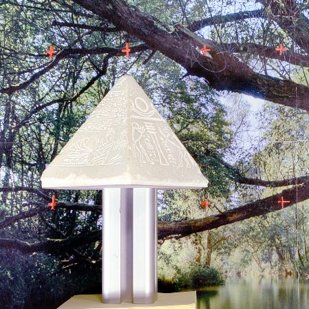
S. Wanner, S. Meister and B. Goldluecke / Datasets and Benchmarks forDensely Sampled 4D Light Fields

  are probabilities for edges [WSG13] for all views. These
  are not only useful for segmentation, but any algorithm
  which might require edge information, and can help with
  comparability since all of these can use the same reference
  edge weights.
• feature_single_view_probabilities.h5:
  The HDF5 dataset Probabilities contains the prediction of
  a random forest classifier trained on a single view of the
  light field without using any feature requiring light field
  information [WSG13].
• feature_depth_probabilities.h5:
  The HDF5 dataset Probabilities contains the prediction of
  a random forest classifier trained on a single view of the
  light field using estimated disparity [WG12] as an addi-
  tional feature [WSG13].
• feature_gt_depth_probabilities.h5:
  The HDF5 dataset Probabilities contains the prediction of
  a random forest classifier trained on a single view of the
  light field using ground truth disparity as an additional
  feature [WSG13].

2.3. Gantry category
In the Gantry category, each scene always provides a sin-
gle main lf.h5 file, which contains an additional HDF5
dataset GT_DEPTH_MASK. This is a binary mask indi-
cating valid regions in the ground truth GT_DEPTH. In-
valid regions in the ground truth disparity have mainly two
causes. First, there might be objects in the scene for which
no 3D data is available, and second, there are parts of the
                                                                      Figure 3: Dataset transparency. Top: center view, bottom
mesh not covered by the structured light scan and thus hav-
                                                                      left: depth of the background, bottom right: depth of the fore-
ing unknown geometry. See section 3.2.1 for details.
                                                                      ground.
   A special case is the light field transparency, which has
two depth channels for a transparent surface and an ob-
ject behind it, respectively. Therefore, there also exist two         3.1. Blender category
mask HDF5 datasets, see figure 3. We believe this is the first
                                                                      For the synthetic scenes, the camera can be moved using
benchmark light field for multi-channel disparity estimation.
                                                                      a script for the Blender engine. As camera parameters can
Here, the HDF5 datasets are named
                                                                      be set arbitrarily and the sensor and movement plane coin-
•   GT_DEPTH_FOREGROUND,                                              cide perfectly, no explicit camera calibration is necessary.
•   GT_DEPTH_BACKGROUND,                                              Instead, the values required for rectification can be derived
•   GT_DEPTH_FOREGROUND_MASK,                                         directly from the internal Blender settings.
•   GT_DEPTH_BACKGROUND_MASK.

3. Generation of the light fields                                     3.2. Gantry category
The process of light field sampling is very similar for both          For the real-world light fields, a Nikon D800 digital camera
the synthetic as well as the real world scenes. The camera is         is mounted on a stepper-motor driven gantry manufactured
moved on a equidistant grid parallel to its own sensor plane          by Physical Instruments. A picture of the setup can be seen
and an image is taken at each grid position. Although not             in figure 4. Accuracy and repositioning error of the gantry
strictly necessary, an odd number of grid positions is used           is well in the micrometer range. The capturing time for a
for each movement direction as there then exists a well-              complete light field depends on the number of images, about
defined center view which makes the processing simpler. An            15 seconds are required per image. As a consequence, this
epipolar rectification on all images is performed to align in-        acquisition method is limited to static scenes. The internal
dividual views to the center one. The source for the internal         camera matrix must be estimated beforehand by capturing
and external camera matrices needed for this rectification de-        images of a calibration pattern and invoking the camera cal-
pends on the capturing system used.                                   ibration algorithms of the OpenCV library, see next section

                                                                                                          c The Eurographics Association 2013.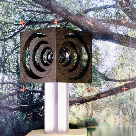
S. Wanner, S. Meister and B. Goldluecke / Datasets and Benchmarks forDensely Sampled 4D Light Fields
Figure 4: Picture of the gantry setup showing a sample ob-
ject placed on the left and the camera mounted on a stepper-
motor on the right.
for details. Experiments have shown that the positioning ac-
curacy of the gantry actually surpasses the pattern based ex-
ternal calibration as long as the differences between the sen-
sor and movement planes are kept minimal.
3.2.1. Ground truth for the Gantry light fields
Ground truth for the real world scenes was generated us-
ing standard pose estimation techniques. First, we acquired
3D polygon meshes for an object in the scene using a
Breuckmann SmartscanHE structured light scanner. The
meshes contain between 2.5 and 8 Million faces with a
stated accuracy of down to 50 micron. The object-to-camera
pose was estimated by hand-picking 2D-to-3D feature points Figure 5: Datasets in the category Gantry. From left to
from the light field center view and the 3D mesh, and right: center view, depth channel, mask which indicates re-
then calculating the external camera matrix using an iter- gions with valid depth information. The ordering of the
ative Levenberg-Marquardt approach from the OpenCV li- datasets is the same as in figure 1.
brary [Bra00]. This method is used for both the internal
and external calibration. An example set of correspondence
points for the scene pyramide can be observed in figure 6. we perform a simple error propagation on the projected point
coordinates. Given an internal camera matrix C and an exter-
The reprojection error for all scenes was typically 0.5 ± nal matrix R, a 3D point ~P = (X,Y, Z, 1) is projected onto the
0.1 pixels. The depth is then defined as the distance between sensor pixel (u v) according to
the sensor plane and the mesh surface visible in each pixel.
The depth projections are computed by importing the mesh
and measured camera parameters into Blender and perform- X
u Y
ing a depth rendering pass. At depth discontinuities (edges) v = C R .
or due to the fact that the meshes’ point density is higher Z
1
than the lateral resolution of the camera, one pixel can con- 1
tain multiple depth cues. In the former case, the pixel was
masked out as an invalid edge pixel and in the latter case, For simplicity, we assume that the camera and object coordi-
the depth of the polygon with the biggest area inside the nate systems coincide, save for an offset tz along the optical
pixel was selected. The error is generally negligible as the axis. Given focal length fx , principal point cx and reprojec-
geometry of the objects is sufficiently smooth at these scales. tion error ∆u, this yields for a pixel on the v = 0 scanline
Smaller regions where the mesh contained holes were also
masked out and not considered for the final evaluations.
fx X
For an accuracy estimation of the acquired ground truth, tz = Z − ,
u − cx
c The Eurographics Association 2013.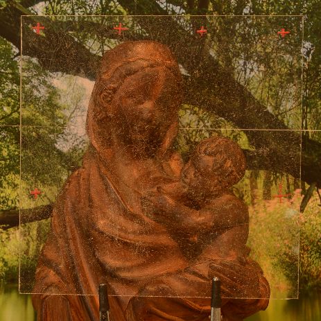
S. Wanner, S. Meister and B. Goldluecke / Datasets and Benchmarks forDensely Sampled 4D Light Fields

                                                                             Algorithm      accuracy      speed         all views
                                                                             ST_CH_G          1.01         slow
                                                                              EPI_C           1.04       medium             yes
                                                                              EPI_S           1.07          fast            yes
                                                                             ST_AV_G          1.12         slow
                                                                             ST_CH_S          1.14          fast
                                                                              EPI_G           1.18         slow
                                                                             ST_AV_S          1.19          fast
                                                                              EPI_L           1.64          fast            yes
                                                                             ST_AV_L          2.72          fast
                                                                             ST_CH_L          3.54          fast
                                                                      Figure 8: Algorithms ranked by average accuracy over all
                                                                      data sets (mean squared error times 100). The computa-
                                                                      tion time depends on exact parameter settings and can vary
                                                                      quite a bit, so we have only roughly classified the algorithms
Figure 6: Selected 2D correspondences for pose estimation
                                                                      as fast (less than five seconds), medium (five seconds to
for the pyramide dataset. In theory, four points are sufficient
                                                                      a minute) and slow (more than a minute). The column all
to estimate the six degrees of freedom of an external camera
                                                                      views indicates whether the algorithm computes the dispar-
calibration matrix, but more points increase the accuracy in
                                                                      ity for all views of the light field in the given time frame or
case of outliers.
                                                                      only for the center view.

resulting in a depth error ∆tz of
                                                                      4.1. Disparity reconstruction algorithms
                      ∂tz         fx X
                ∆tz =     ∆u =           ∆u.                          The following is a description of the methods for disparity
                      ∂u       (cx − u)2
                                                                      reconstruction which are currently implemented in the test
Calculations for pixels outside of the center scanline are per-       suite and ranked in the results. See figure 8 for an overview,
formed analogously. The error estimate above depends on               and figure 7 for detailed results.
the distance of the pixel from the camera’s principal point.
As the observed objects are rigid, we assume that the dis-               For all methods, we compute results from local data terms
tance error ∆tz between camera and object corresponds to              separately, and compared the same regularization schemes
the minimum observed ∆tz among the selected 2D-3D cor-                where possible. In the test suite, many more regularization
respondences. For all gantry scenes, this value is in the range       schemes are implemented and are ready to use. However,
of 1mm so we assume this to be the approximate accuracy of            comparisons are restricted to a subset of simple regularizers,
our ground truth.                                                     since usually the data term has more influence on the quality
                                                                      of the result.

4. Evaluation
                                                                      4.1.1. EPI-based methods
The benchmark data sets are accompanied by a test suite
which is coded in CUDA / C++ and which contains a num-                A number of methods exist which estimate disparity by com-
ber of implementations for recent light field analysis algo-          puting the orientation of line patterns on the epipolar plane
rithms. Complete source code is available, and it is our in-          images [BBM87, CKS∗ 05, WG12]. They make use of the
tention to improve and update the test suite over the next            well known fact that a 3D point is projected onto a line
years. As such, the list of algorithms and results below is           whose slope is related to the distance of the point to the ob-
only a snapshot of the current implementation. For example,           server.
an implementation of the multiview graph cut scene recon-
                                                                         For the benchmark suite, we implemented a number of
struction [KZ02] is scheduled for an upcoming version. We
                                                                      schemes of varying complexity. First, we start with the
will regularly publish benchmark results for the newest im-
                                                                      purely local method EPI_L, which estimates orientation us-
plementation.
                                                                      ing an Eigensystem analysis of the structure tensor [WG12].
   The project will be hosted on SourceForge, and others are          The second method, EPI_S, just performs a TV-L2 denois-
of course invited to contribute more algorithms for compari-          ing of this result [WG13], while EPI_G employs a glob-
son and evaluation, but this is not a requirement to get listed       ally optimal labeling scheme [WG12]. Finally, the method
in the results. Instead, we will provide a method indepen-            EPI_C performs a constrained denoising on each epipolar
dent from the test suite code to submit results and have them         plane image, which takes into account occlusion ordering
ranked in the respective tables.                                      constraints [GW13].

                                                                                                          c The Eurographics Association 2013.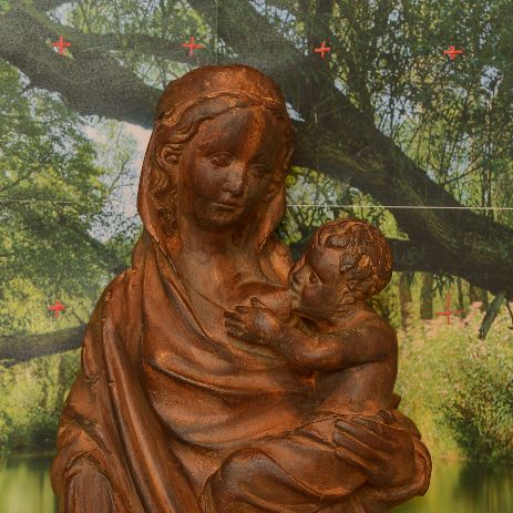
S. Wanner, S. Meister and B. Goldluecke / Datasets and Benchmarks forDensely Sampled 4D Light Fields

  lightfield       EPI_L           EPI_S      EPI_C        EPI_G     ST_AV_L    ST_AV_S    ST_AV_G       ST_CH_L       ST_CH_S      ST_CH_G
  buddha            0.81            0.57       0.55         0.62       1.20       0.78       0.90          1.01          0.67         0.80
  buddha2           1.22            0.87       0.87         0.89       2.26       1.05       0.68          3.08          1.31         0.75
  horses            3.60            2.12       2.21         2.67       5.29       1.85       1.00          6.14          2.12         1.06
  medieval          1.69            1.15       1.10         1.24       7.22       0.91       0.76          12.14         1.08         0.79
  mona              1.15            0.90       0.82         0.93       2.25       1.05       0.79          2.28          1.02         0.81
  papillon          3.95            2.26       2.52         2.48       4.84       2.92       3.65          4.85          2.57         3.10
  stillLife         3.94            3.06       2.61         3.37       5.08       4.23       4.04          4.48          3.36         3.22
  couple            0.40            0.18       0.16         0.19       0.60       0.24       0.30          1.10          0.24         0.30
  cube              1.27            0.85       0.82         0.87       1.28       0.51       0.56          2.25          0.51         0.55
  maria             0.19            0.10       0.10         0.11       0.34       0.11       0.11          0.51          0.11         0.11
  pyramide          0.56            0.38       0.38         0.39       0.72       0.42       0.42          1.30          0.43         0.42
  statue            0.88            0.33       0.29         0.35       1.56       0.21       0.21          3.39          0.29         0.21
  average           1.64            1.07       1.04         1.18       2.72       1.19       1.12          3.54          1.14         1.01

Figure 7: Detailed evaluation of all disparity estimation algorithms described in section 4 on all of the data sets in our
benchmark. The values in the table show the mean squared error in pixels times 100, i.e. a value of “0.81” means that the mean
squared error in pixels is “0.0081”. See text for a discussion.

4.1.2. Multi-view stereo                                                         in [PCBC10]. The global optimization results can be found
                                                                                 under algorithms ST_AV_G and ST_CH_G.
We compute a simple local stereo matching cost for a sin-
gle view as follows. Let V = {(s1 ,t1 ), ..., (sN ,tN )} be the
set of N view points with corresponding images I1 , ..., IN ,
with (sc ,tc ) being the location of the current view Ic for                     4.1.3. Results and discussion
which the cost function is being computed. We then choose
                                                                                 At the moment of writing, the most accurate method over all
a set Λ of 64 disparity labels within an appropriate range.
                                                                                 data sets is the straight-forward global stereo ST_CH_G. In-
For our test we choose equidistant labels within the ground
                                                                                 terestingly, using only a subset of input views gives more ac-
truth range for optimal results. The local cost ρAV (x, l) for
                                                                                 curate results after global optimization, while the data term
label l ∈ Λ at location x ∈ Ic computed on all neighbouring
                                                                                 accuracy is clearly worse. However, global stereo takes sev-
views is then given by
                                                                                 eral minutes to compute. Among the real-time capable meth-
   ρAV (x, l) :=        ∑          min(ε, kIn (x + lvn ) − Ic (x)k),      (3)    ods, EPI_S and the ST_S methods perform comparably well.
                     (sn ,tn )∈V                                                 The difference is that the stereo methods only compute the
                                                                                 disparity map for the center view in real-time, while EPI_S
where vn := (sn − sc ,tn − tc ) is the view point displacement                   recovers disparity for all views simultaneously, which might
and ε > 0 is a cap on the error to suppress outliers. To test                    be interesting for further processing. Furthermore, EPI_S
the influence of the number of views, we also compute a cost                     and EPI_C do not discretize the disparity space, so accuracy
function on a “crosshair” of view points along the s- and t-                     is independent of computation time.
axis from the view (sc ,tc ), which is given by
                                                                                    As usual, overall performance depends very much on pa-
        ρCH (x, l) :=              ∑         kIn (x + lvn ) − Ic (x)k .   (4)
                              (sn ,tn )∈V
                                                                                 rameter settings, for the results here, we did a parameter
                          sn =sc or tn =tc                                       search to find the optimum for all methods on each data set
In effect, this cost function thus uses exactly the same num-                    separately. In the future, we would like to do a second run
ber of views as required for the local structure tensor of the                   with equal parameter values for each data set, which might
center view. The results of these two purely local methods                       turn out quite interesting. These results will also be available
can be found under ST_AV_L for all views, and ST_CH_L                            online.
for all views or just a crosshair, respectively.
   Results of both multiview dataterms are denoised with a
simple TV-L2 scheme, algorithms ST_AV_S and ST_CH_S.                             4.2. Multiple layer estimation
Finally, they were also integrated into a global energy func-
tional                                                                           One of our data sets is special in that it contains a transpar-
                          Z                            Z                         ent surface, so there are two disparity channels, one for the
               E(u) =           ρ(x, u(x)) dx + λ           |Du|          (5)    transparent surface and one for the object behind it, see fig-
                            Ω                           Ω                        ure 3. For this case, we currently only have one method im-
for a labeling function u : Ω → Λ on the image domain Ω,                         plemented [Ano13], and we are quite interested in whether
which is solved to global optimality using the method                            it can be done better.

c The Eurographics Association 2013.
S. Wanner, S. Meister and B. Goldluecke / Datasets and Benchmarks forDensely Sampled 4D Light Fields

4.3. Light field labeling algorithms                                   [CKS∗ 05] C RIMINISI A., K ANG S., S WAMINATHAN R.,
                                                                         S ZELISKI R., A NANDAN P.: Extracting layers and analyz-
For labeling, we have implemented all algorithms which are               ing their specular properties using epipolar-plane-image analysis.
described in [WSG13]. The results are equivalent, and we                 Computer vision and image understanding 97, 1 (2005), 51–85.
refer to this work for details. Test scripts to re-generate all          6
their results are included with the source code.                       [EM03] E SEDOGLU S., M ARCH R.: Segmentation with Depth
                                                                         but Without Detecting Junctions. Journal of Mathematical Imag-
                                                                         ing and Vision 18, 1 (2003), 7–15. 2
5. Conclusion                                                          [GW13] G OLDLUECKE B., WANNER S.: The Variational Struc-
We have introduced a new benchmark database of densely                   ture of Disparity and Regularization of 4D Light Fields. In
                                                                         Proc. International Conference on Computer Vision and Pattern
sampled light fields for the evaluation of light field analysis          Recognition (2013). 6
algorithms. The database consists of two categories. In the
                                                                       [KSS12] KOWDLE A., S INHA S., S ZELISKI R.: Multiple View
first category, there are artificial light fields rendered with          Object Cosegmentation using Appearance and Stereo Cues. In
Blender [Ble], which provide ground truth disparities for all            Proc. European Conference on Computer Vision (2012). 2
views. For some of those light fields, we additionally pro-            [KZ02] KOLMOGOROV V., Z ABIH R.: Multi-camera Scene Re-
vide ground truth labels for object segmentation. In the sec-            construction via Graph Cuts. In Proc. European Conference on
ond category, there are real-world scenes captured using a               Computer Vision (2002), pp. 82–96. 6
single camera mounted on a gantry, for which we provide                [LH96] L EVOY M., H ANRAHAN P.: Light field rendering. In
(partial) ground truth disparity data for the center view, gen-          Proc. SIGGRAPH (1996), pp. 31–42. 1
erated via fitting a mesh from a structured light scan to the          [LNA∗ 06] L EVOY M., N G R., A DAMS A., F OOTER M.,
views. A large contribution is the source code for an ex-                H OROWITZ M.: Light field microscopy. ACM Transactions on
tensive evaluation of reference algorithms from multi-view               Graphics (TOG) 25, 3 (2006), 924–934. 1
stereo, epipolar plane image analysis and segmentation on              [Ng06] N G R.: Digital Light Field Photography. PhD thesis,
the entire database.                                                     Stanford University, 2006. Note: thesis led to commercial light
                                                                         field camera, see also www.lytro.com. 1
   The paper only describes a current snapshot for the                 [PCBC10] P OCK T., C REMERS D., B ISCHOF H., C HAMBOLLE
database, and explains only a subset of the available source             A.: Global Solutions of Variational Models with Convex Regu-
code, which offers many more optimization models and data                larization. SIAM Journal on Imaging Sciences (2010). 7
terms. Both will be regularly updated, in particular we plan           [PW10] P ERWASS C., W IETZKE L.: The Next Generation of
new light fields recorded with a plenoptic camera and with               Photography, 2010. www.raytrix.de. 1
available ground truth depth data, as well as extensions of            [SHH07] S TEIN A., H OIEM D., H EBERT M.: Learning to Find
the code base with reference implementations of more multi-              Object Boundaries Using Motion Cues. In Proc. International
view reconstruction algorithms.                                          Conference on Computer Vision (2007). 2
                                                                       [The10] T HE HDF G ROUP: Hierarchical data format version 5,
                                                                         2000-2010. URL: http://www.hdfgroup.org/HDF5. 2
6. Acknowledgement
                                                                       [WG12] WANNER S., G OLDLUECKE B.: Globally consistent
We thank Julie Digne from the LIRIS laboratory of the                    depth labeling of 4D light fields. In Proc. International Con-
Claude-Bernard University for providing multiple of the                  ference on Computer Vision and Pattern Recognition (2012),
                                                                         pp. 41–48. 4, 6
scanned objects. We also thank Susanne Krömker from the
Visualization and Numerical Geometry Group of the IWR,                 [WG13] WANNER S., G OLDLUECKE B.: Variational Light
                                                                         Field Analysis for Disparity Estimation and Super-Resolution.
University of Heidelberg as well as the Heidelberg Gradu-                IEEE Transactions on Pattern Analysis and Machine Intelligence
ate School of Mathetmatical and Computational Methods for                (2013). 6
the Sciences (HGS MathComp) for providing us with high                 [WJV∗ 05] W ILBURN B., J OSHI N., VAISH V., TALVALA E.-V.,
precission 3D scans and support.                                         A NTUNEZ E., BARTH A., A DAMS A., H OROWITZ M., L EVOY
                                                                         M.: High performance imaging using large camera arrays. ACM
                                                                         Transactions on Graphics 24 (July 2005), 765–776. 1
References
                                                                       [WSG13] WANNER S., S TRAEHLE C., G OLDLUECKE B.: Glob-
[AB91] A DELSON E., B ERGEN J.: The plenoptic function and               ally Consistent Multi-Label Assignment on the Ray Space of 4D
  the elements of early vision. Computational models of visual           Light Fields. In Proc. International Conference on Computer Vi-
  processing 1 (1991). 1                                                 sion and Pattern Recognition (2013). 2, 4, 8
[Ano13]   A NONYMOUS: Anonymous. In under review (2013). 7
[BBM87] B OLLES R., BAKER H., M ARIMONT D.: Epipolar-
  plane image analysis: An approach to determining structure from
  motion. International Journal of Computer Vision 1, 1 (1987),
  7–55. 6
[Ble]   Blender Foundation. www.blender.org. 2, 8
[Bra00] B RADSKI G.: The OpenCV Library. Dr. Dobb’s Journal
  of Software Tools (2000). 5

                                                                                                             c The Eurographics Association 2013.
You can also read