Efficiency or resiliency? Corporate choice between operational and financial hedging (Preliminary and Incomplete - Do not circulate or quote)
←
→
Page content transcription
If your browser does not render page correctly, please read the page content below
Efficiency or resiliency?
     Corporate choice between operational and financial hedging
      (Preliminary and Incomplete - Do not circulate or quote)

    Viral V. Acharya∗          Heitor Almeida†             Yakov Amihud‡              Ping Liu§

                                       December 2020

                                            Abstract
     We study the corporate choice between financial efficiency and operational resilience.
     Firms substitute between saving cash for financial hedging, which mitigates the risk
     of financial default, and spending on operational hedging which mitigates the risk
     of operational default and failure to deliver on their obligations to customers. This
     tradeoff is particularly strong for financially constrained firms and is reflected in a
     positive correlation between operational spread (markup) and financial leverage or
     credit risk. We present empirical evidence supporting this correlation, the effect being
     stronger for constrained firms.

     Keywords: financial default, operational default, liquidity, financial
     constraints, risk management
     JEL: G31, G32, G33

∗
  New York University, Stern School of Business, NBER, and CEPR: vacharya@stern.nyu.edu.
†
  University of Illinois at Urbana-Champaign, Gies College of Business, NBER: halmeida@illinois.edu.
‡
  New York University, Stern School of Business: yamihud@stern.nyu.edu.
§
  Purdue University, Krannert School of Management: liu2554@purdue.edu.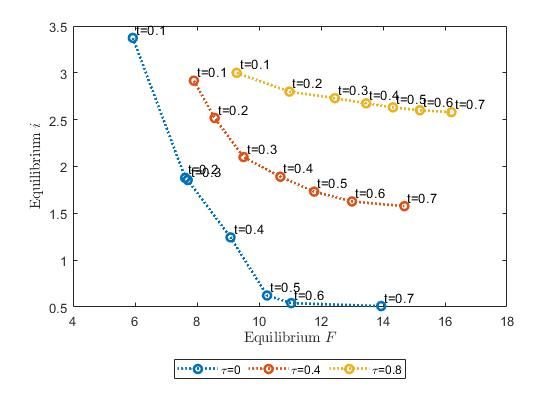
1.      Introduction

The Covid-19 crisis has raised the issue of corporate resilience to shocks following disruptions
in supply chains which adversely affect operations. Companies tackle such negative supply-
chain shocks by operationally hedging against them. This includes diversifying the supply
chains by allocating resources to increase the pool of suppliers and shifting some of them to
nearby, more secure locations; maintaining backup capacity; and, holding excess inventory.
In essence, companies endure a higher cost of production — through holding spare capacity
and excess inventory, and rearranging their supply chains — in order to mitigate the risk of
operational disruption.
      A global survey by Institute for Supply Management finds that by the end of May
2020, 97% of organizations reported that they would be or had already been impacted by
coronavirus-induced supply-chain disruptions.1 Consequently, U.S. manufacturing is operat-
ing at 74% of normal capacity while in Europe capacity is at 64%. The survey also finds that
while firms in North America report that operations have or are likely to have inventory to
support current operations, confidence has declined to 64% in the U.S., 49% in Mexico and
55% in Canada. In Japan and Korea too, many firms are not confident that they will have
sufficient inventory for Q4; and, almost one-half of the firms are holding inventory more than
usual. In response, 29% of organizations are planning or have begun to re-shore or near-
shore some or most operations.2 However, such operational resiliency is not being favored
by all firms as several corporate chief executive officers (CEOs) and investors contend that
  1
     https://www.prnewswire.com/news-releases/covid-19-survey-round-3-supply-chain-disr
uptions-continue-globally-301096403.html. See also “Businesses are proving quite resilient to the
pandemic”, The Economist, May 16th 2020, and “From ‘just in time’ to ‘just in case’”, Financial Times,
May 4th 2020.
   2
     “Reshoring” and “nearshoring” is the process of bringing the manufacturing of goods to the firm’s
country or a country nearby, respectively.

                                                  1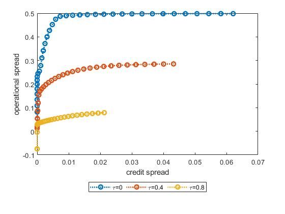
operational hedging is costly and occurs at the cost of financial efficiency.3
      Our paper studies one aspect of the tension between operation resiliency and financial
efficiency, viz., the tradeoff between the firm’s allocation of cash to operational hedging and
to the prevention of financial distress. While operational hedging may be beneficial on its
own, it may compete for resources with the firm’s demand for financial hedging. The need
to optimally balance these two hedging needs — operational hedging and financial hedging
— can help explain the lack of operational resilience in some firms.
      In our theoretical setting, a levered company faces two important risks. First, it faces a
risk of financial default, because cash flows from assets in place are risky. Second, the firm
faces operational risk due to an existing commitment to deliver goods to costumers. The
two risks — financial default and operational default — are possibly related. For example,
an aggregate shock may affect both the firm’s cash flows, possibly enough to induce financial
default, and the firm’s suppliers, who may be unable to deliver to the firm, causing the firm
to default on its contract to deliver goods to its customers. Both financial and operational
defaults lead to a loss in the franchise value of the firm.
      The firm can use its cash inflow to build up cash buffers and mitigate the risk of financial
default. The firm can also use the cash inflow to increase the likelihood that it will deliver
on its promise to customers by allocating resources to operational hedging that includes
greater expenses on supply chains, maintaining backup capacity, and holding excess inven-
tory. Naturally, such operational hedging raises the firm’s cost of production or reduces its
operational spread, viz., the “markup” or the price-to-cost margin per unit. Even an unlev-
ered firm will in general optimally choose an interior level of operational hedging in order
to protect its profitability while recognizing that an operational default leads to a loss of its
franchise value.
  3
      https://www.ft.com/content/4ee0817a-809f-11ea-b0fb-13524ae1056b

                                                 2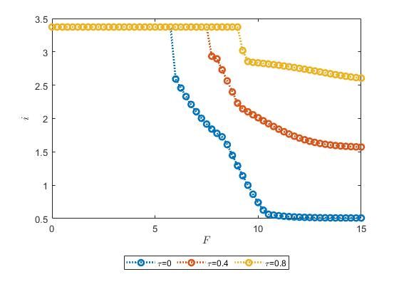
Because operational hedging reduces the risk of delivering to the firm’s customers, it
can potentially also reduce the risk of financial default by increasing the firm’s capacity
to raise financing against future cash flows. However, this is feasible only if the firm can
pledge the benefits of operational hedging to outside investors. For firms that are financially
constrained, such pledgeability may be low; in turn, financial and operating hedging become
substitutes: the firm must decide between using cash to mitigate the risk of financial default,
or spending cash on contracting with higher-cost suppliers, holding excess inventory, or
maintaining spare capacity.
   Our principal theoretical result is that for a financially constrained firm, the optimal
amount of operational hedging decreases with the credit spread which is increasing in fi-
nancial default risk. Operational hedging also reduces the operational spread as it increases
firm’s cost of production. In other words, the firm optimally sacrifices operational resiliency
for financial efficiency. This creates a negative relation between the credit spread and the
operational spread. More financial hedging that reduces the credit spread also reduces oper-
ational hedging and this is reflected in a wider operational spread. Similarly, our model also
predicts that higher existing leverage is associated with a wider operational spread. This
positive relation between leverage and operational spread is also pronounced for financially
constrained firms since unconstrained firms can engage in operational hedging and simulta-
neously pledge superior operating cash flows to avoid default should there be a shortfall in
cash.
   We provide empirical tests of our model’s prediction on the tradeoff between operational
hedging and credit risk, or specifically, between the operational spread (or markup) and
financial leverage or measures of credit risk, and relate that to firms’ financially constraint.
   We start by documenting that markup or operational spread is correlated with proxies
for operational hedging in the expected way: higher inventory and greater supply chain

                                               3
diversification reduce the operational spread. This supports the use of operational spread
as a summary measure of the extent of operational hedging that the firm engages in. We
then examine whether leverage and credit risk are correlated with the operational spread in
the way predicted by our model. We find that higher leverage and higher credit risk, mea-
sured using Altman’s z-score, which necessitate allocation of cash to financial hedging, are
positively related to the operational spread or markup, implying a reduction in operational
hedging. To gauge the economic significance of the effect, one standard deviation increase in
the firm’s negative z-score raises the firm’s markup by 0.04 standard deviation, or 13% of the
sample median markup. We find that the positive relation between the operational spread
and leverage is stronger for the short-term portion of the long-term debt which matures in
the next two years. Higher short-term portion of the long-term debt raises the operational
leverage about twice as strongly as does long-term debt. This is consistent with our model
by which the near-term need to avert financial default diverts funds from longer-term op-
erational hedging, and this is reflected in a wider operational spread when there is more
short-term debt due. Notably, the near-term of debt is exogenous to the current state of the
firm, having been determined in the past when the long-term debt was issued.
   We conduct two tests to address concerns about the usefulness of measures of financial
constraints and about the endogeneity of leverage. First, we exploit an exogenous shock to
credit supply to firms following Chodorow-Reich (2014), who studies the negative impact of
the subprime mortgage crisis and Lehman Brothers’ collapse on lenders’ abilities to extend
credit to borrowers. A firms’s exposure to this shock, in terms of its relationship banks
being affected by the shock, reflects a tightening of its financing constraint. We find that
exposed firms that were more highly levered prior to the crisis reduced operational hedging
by more than less exposed firms. This test uses time-series variation in financing constraints
to measure our predicted tension between operational hedging and financial hedging. This

                                              4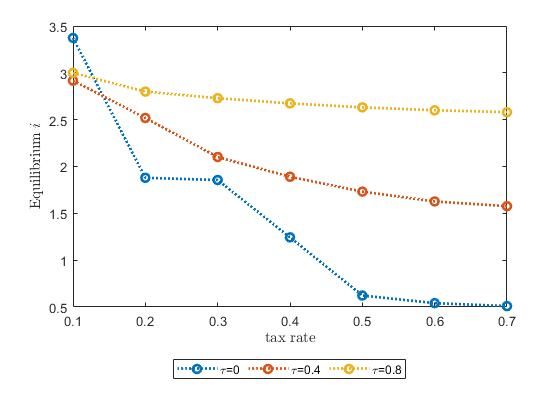
test also helps address concerns about the endogeneity of leverage in that existing literature
on the impact of the financial crisis has shown that pre-crisis leverage is an important
determinant of real effects post-crisis through a liquidity channel (e.g., Giroud and Mueller,
2016)
   Second, we exploit an exogenous increase in the inducement to raise debt following Heider
and Ljungqvist (2015) who find that increases in state taxes induced increases in leverage of
the exposed firms. By our model, these firms should reduce operational hedging, reflected
in widening of their operational spread or markup. This test can help identify the effect
of leverage on operational hedging under the reasonable assumption that changes in state
taxes do not directly affect operational hedging. We find that an increase in state tax was
associated with an increase in the operational spread which indicates a reduction in expenses
on operational hedging. We further test our model’s prediction that leverage more strongly
affects the operational spread in financially-constrained firms. We find that the positive
effect of increased state taxes on operational leverage prevails for constrained firms, using
various common measures of financial constraint.
   Our paper is related to studies of the real effects of financing constraints (see Stein
(2003) for a review) which show that financing frictions can affect investment decisions and
employment (Lemmon and Roberts, 2010; Duchin et al., 2010; Almeida et al., 2012; Giroud
and Mueller, 2016). The literature also studies the effect of financial constraints and financial
distress on financial policies such as cash, credit lines, and risk management (e.g., Almeida
et al., 2004; Sufi, 2009; Bolton et al., 2011; Acharya et al., 2012). Our paper also relates
closely to those of Rampini and Viswanathan (2010) and Rampini et al. (2014), who show
that more constrained or distressed firms may reduce their engagement in risk management in
order to preserve debt capacity for investment and other current expenditures. These studies
focus on financial hedging through derivatives while our focus is on operational hedging. Our

                                               5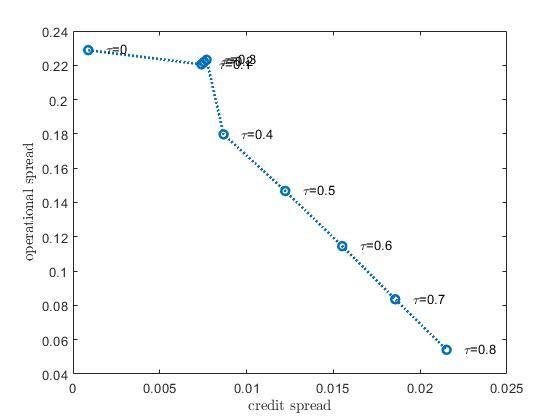
paper also relates to Froot et al. (1993), who propose a theory for the rationale for corporate
hedging. In Froot et al. (1993), hedging against cash shortfalls helps the firm mitigate the
risk of not being able to finance valuable investment opportunities. In our model, however,
operational hedging is not a means to avoid financing shortfall but it is rather the other
way around: A shortfall of cash that presents a financial default risk reduces the resources
allocated to operational hedging.
     Studies of the relationship between a firm’s liquidity position and its markup (e.g.,
Gilchrist et al., 2017; Dou and Ji, 2020) propose that financially constrained firms that
need to increase short-term profits may raise their product price and thus their markup.
Such an ability to extract higher profit by raising prices implicitly assumes market power.
Our analysis controls for market power which is known to be positively associated with the
firm’s markup. We find that the effect of market power on the operational spread is larger
for constrained firms. Yet we find that our model’s predicted positive association between
operational spread and leverage or credit risk persists after controlling for market power.
     Broadly speaking, our contribution in this paper is to study both theoretically and em-
pirically the determinants of operational hedging and its tradeoff with financial hedging,
especially for financially-constrained firms. To our best knowledge, the positive relation-
ship between operational spread (markup) and financial leverage or credit risk has not been
documented in the literature.

2.      The model

2.1     Model setup

This section develops a model of a levered firm’s optimal operational hedging policy in the
presence of costly financial default (default on debt service) and operational default (default

                                              6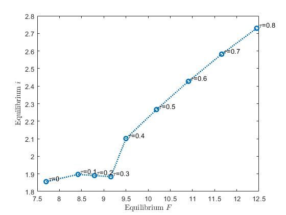
on the supplier contract). Our main goal is to show that the firm faces a tension between
operational hedging and financial hedging, where we model financial hedging as the firm
saving cash in order to avoid default on its debt maturing before the settlement date of
supply contracts with its customers.
   Our model introduces operational hedging in the setting of Acharya et al. (2012) who
study the impact of credit risk on the firm’ s cash holding. The model features a single-
levered firm with existing debt F in a three-period economy: t = 0, 1, 2. The firm has assets
in place that generate a cash flow xt at each period t = 0, 1. x2 represents the franchise
or the continuation value. Additionally, the firm has an outstanding supplier contract that
stipulates a delivery of I units of goods at unit price p at t = 2. Our goal is to analyze the
tension between the firm’s cash holding and operational hedging decisions to avoid financial
and operational defaults, respectively.
   For our purpose, it is important to introduce a random shock u that affects both the firm’s
cash flow at t = 1 and its capacity to fulfill the supplier contract. Specifically, the firm’s
cash flow from assets in place at t = 1 is given by x1 = x̄1 + u, and its production capacity
is reduced from I to (1 − δ(u))I, where δ(u) is decreasing and convex in u with continuous
and finite first and second order derivatives. The probability distribution of u is given by the
density function g(u) with support [0, ∞), the associated cumulative distribution function
being G(u) and the hazard function h(u) being defined as

                                                  g(u)
                                       h(u) =            .                                 (2.1)
                                                1 − G(u)

To derive analytical results, we assume that u is exponentially distributed on [0, ∞) with
density function g(u) = αe−αu . Then the cumulative distribution function G(u) = 1 − e−αu
and the hazard function h(u) is a constant α. Figure 1 illustrates the timeline of the model.

                                                7
2
p[(1 − δ(u))I + i] + x2 realized.
2
t [1 − δ(u)]I + i < I,
0 1 operational default,
cash flow x0 , cash flow x1 , p[(1 − δ(u))I + i] + (1 − λ)x2 realized.
Operational hedging amount i Debt F matures.
is chosen.
Production cost K(I + i) is sunk. x0 + x̄1 + u < F + K(I + i),
financial default
Figure 1: The timeline of the model
At date t = 0, the assets in place generate a positive cash flow x0 > 0. At this time, the
firm starts producing I units of goods scheduled for delivery at t = 2. Moreover, the firm can
choose to hedge the operational risk by investing in excess inventory i, resulting in the total
units of delivered goods being (1 − δ(u))I + i. Note that i can also be interpreted as spare
production capacity. The cost of the production and operational hedging is summarized by
an increasing and convex cost function K(I + i) with continuous and finite first and second
order derivatives. We assume that the firm is a price-taker in its supplier contracts. We also
make the following assumption regarding the unit product price p and the marginal cost of
production commitment I:
Assumption 2.1.
p > K 0 (I) . (2.2)
Assumption 2.1 says that the firm enjoys some positive markup over the marginal cost of
the production commitment. Since the production cost function K is convex, this assumption
says that the firm can potentially choose a positive hedging policy i and still enjoy a positive
marginal profit from the supplier contract. Market frictions preclude the firm from accessing
8outside financing, so that the firm’s disposable cash at date-0 comes entirely from its internal
cash flow. Thus, the cash reserve is c = x0 − K(I + i).
At date t = 1, the firm must make a debt payment of F , which is assumed to be
predetermined (a legacy of the past). We assume that debt cannot be renegotiated due
to high bargaining costs; for example, it might be held by dispersed bondholders prone to
coordination problems. Failure to repay the debt in full at t = 1 results in financial default
and liquidation, in which case future cash flow from the contractual delivery investment,
p[(1 − δ(u)) + i], and franchise value, x2 , are lost. Since the period-1 cash flow, x1 , is
random, there is no assurance that the firm has enough liquidity to repay the debt in full.
Moreover, failure to deliver I units of goods results in operational default, also leading to a
loss of the franchise value, x2 , by a portion λ ∈ [0, 1). This can be interpreted as, for example,
a loss of reputation with some of its customers who can switch to alternate suppliers.
Due to market frictions, external financing is unavailable also at t = 1, and hence the
debt payment must be made out of the firm’s internal funds. The financing friction gives
rise to a tension between financial hedging versus operational hedging decisions at t = 0:
On the one hand, the firm has incentive to spend on excess inventory i, to hedge against
the operational shock and reduce the probability of operational default; on the other hand,
such operational hedging worsens its liquidity position between periods 0 and 1, thereby
increasing the probability of a future cash shortfall and financial default.
2.2 Discussion
Before proceeding further, we want to stress that the exact specification of the model can vary
widely without affecting the results qualitatively, as long as two assumptions are satisfied.
First, default involves deadweight costs. Although we assume that all future cash flows are
lost in default, an extension to a partial loss is straightforward. Second, external financing
9cannot be raised against the full income from the supplier contract settlement at date-2. If
the firm can pledge a large enough fraction of its income from fulfilling the supplier contract as
collateral, then current and future cash holdings can be viewed as time substitutes, and there
is no role for precautionary savings of cash. As a result, the tension between financial hedging
and operational hedging breaks down. In reality, the condition of partial pledgeability is
likely to be universally met. While the base case model assumes that external financing is
prohibited, Section 3.1 extends the model by allowing the firm to borrow up to a certain
fraction τ of its cash flow from contract settlement at t = 2, and shows that our main results
hold as long as financing constraints are sufficiently binding, i.e., τ is sufficiently small.
A related feature in our model is that the outstanding debt matures before the supplier
contract settlement date, giving rise to a maturity mismatch between debt contract and
supplier contract. Effectively, the cash flow from the supplier contract can neither be fully
pledged nor used as cash to cover debt obligations. In practice, supplier contracts often
stipulate a considerable elapsed time from initiation to settlement, especially in the case of
durable goods industry. Meanwhile, firms often have to borrow short-term debt or draw
down their credit lines to finance their working capital needs during the production process.
What is crucial here is that the shock at t = 1 can be severe enough to make the cash flow at
date-1 fall short of the debt contract obligation and make the production capacity fall short
of the supplier contract obligation. This creates the needs for both financial and operational
hedging. The two needs compete with each other in our model. Although we assume a single
uncertainty state affects both the cash flows from assets in place and the ability to fulfill the
supplier contract, extending our model to different sources of uncertainties is possible.
In general, in addition to saving and investing, firms can also distribute some of the cash
to their shareholders. Fixed, pre-committed dividends at t = 0 amount to a reduction in
the net cash flow x0 , and can be easily incorporated in the model. Although modeling an
10optimal dividend policy at t = 0 would complicate the analysis considerably by introducing
a second choice variable, the intuition on the effect of optimal dividends is as follows. Most
firms in the model would choose not to pay any dividend at either date-0 or date-1. This is
because the cash can be saved to avoid costly financial bankruptcy, or it can be invested in
inventory or spare production capacity to weather operational disruptions. However, if the
firm is very risky, meaning the shock at t = 1 is sufficiently detrimental to the firm’s cash
flow x1 and production capacity, the precautionary motive for saving cash and investment
in operational hedging can be dominated by the incentives to engage in asset substitution,
i.e., to pay out a large immediate dividend at the expense of making the firm even riskier
(Jensen and Meckling, 1976). In our base-case model, we assume that in order to prevent
such behavior, discretionary dividends are prohibited by debt covenants.
Moreover, if the firm has access to external capital at t = 0, it can choose to raise
additional capital at that time to invest in operational hedging and/or cash holdings. Selling
equity can be viewed as making a negative dividend payment. By the same logic as above,
in our model a firm may find it desirable to raise equity, as long as the marginal value of
an additional dollar of operational hedging is greater than one. However, if the firm is very
risky, instead of contributing the proceeds from additional equity issuance to the operational
hedging, shareholders would have incentives to pay themselves a dividend and not engage in
operational risk management.
Finally, shareholders may find it optimal to raise debt maturing at t = 1 that is more
senior than the existing debt and invest in operational hedging. This occurs when sensitivity
of function δ(u) with respect to u and the cost of operational default (captured by λ) are
both sufficiently high.4 In our base case model, we assume that financing constraints at t = 0
4
By contrast, as in Acharya et al. (2012), raising debt maturing at t = 1 solely to increase the cash reserve
is value-neutral in this setting, as the increase in cash is exactly offset by the increase in the required debt
repayment (i.e., cash is negative debt in this setting of “short-term” debt).
11preclude the firm from accessing any additional financing. Explicitly modeling endogenous
capital structure polices at date-0 is an interesting extension of our model. In Section 4.2,
we allow for tax shields of debt and numerically solve for the firm’s optimal debt policy (F )
at date-0 as a function of the pledgeability of its cash flow and the corporate tax rate.
2.3 Optimal hedging policies
In general, the firm has a positive amount of existing debt (F > 0). At date 0, the firm faces
the following trade-off between investing its cash in the operational hedging and retaining it
until the next period. The firm’s optimal hedging policies depend on the relative likelihood
of financial default and operational default, as will be shown below.
The amount of cash available for debt service at date 1 is x0 − K(I + i) + x1 , where
x0 − K(I + i) is the cash reserve and x1 = x̄1 + u is the interim-period cash flow from assets.
The “financial default boundary”, uF , is the minimum cash flow shock that allows the firm
to repay F in full and avoid default:
uF = F + K(I + i) − x0 − x̄1
= F̄ + K(I + i) , (2.3)
where F̄ = F − x0 − x̄1 is the net debt, i.e., debt minus date 0 and 1 predictable cash flows.
The financial default boundary uF increases with the level of net debt (F̄ ) and operational
hedging amount (i). For all realizations of u between 0 and uF , the firm defaults on its debt
contract and equity holders are left with nothing.
We also allow the firm to default on the supplier contract. The amount of goods that
the firm can deliver at date-2 is (1 − δ(u))I + i. If this amount is less than the production
commitment I, the firm defaults on the supplier contract. Correspondingly, the “operational
12default boundary”, uO , is the minimum shock that allows the firm to deliver its contractual
amount of goods in full and avoid operational default:
(1 − δ(uO ))I + i = I, or
−1 i
uO = δ . (2.4)
I
Since the loss function δ is decreasing in u, its inverse function δ −1 is decreasing in i. This
means that the operational default boundary uO is decreasing with i, the amount of op-
erational hedging the firm chose at date-0. In this sense, operational hedging reduces the
operational default risk. For all realizations of u between 0 and uO , the firm defaults on its
supplier contract and equity holders lose a portion λ of the franchise value x2 .
Define D(i, F̄ ) as the difference between financial and operational default thresholds for
given net debt level F̄ and operational hedging policy i:
−1 i
D(i, F̄ ) ≡ uF − uO = F̄ + K(I + i) − δ . (2.5)
I
D(i, F̄ ) is continuously differentiable in both i and F̄ with partial derivatives:
∂D 1
= K 0 (I + i) − 0 , (2.6a)
∂i Iδ (uO )
∂D
=1. (2.6b)
∂ F̄
Note that ∂D
∂ ī
> 0 because K 0 (I + i) > 0 and δ 0 (u) < 0 by assumption.
132.3.1 Benchmark: Optimal hedging policy when F = 0
Consider first a benchmark case when the debt level F = 0. In this case, financial default
is irrelevant: uF = 0. In this case, the firm will choose the hedging policy ī that maximizes
the unlevered date-0 equity value:
Z ∞ h i Z uO
Ē = x0 − K(I + i) + x̄1 + u + p [(1 − δ(u))I + i] + x2 g(u)du − λx2 g(u)du . (2.7)
0 0
The last term of Equation (2.7) reflects the proportional loss of franchise value in case of
operational default. The first-order condition is
∂ Ē g(uO )
= p − K 0 (I + i) − λx2 0 =0, (2.8)
∂i Iδ (uO )
where uO = δ −1 i
I
. Define ī being the solution for the first-order condition (2.8). In
Appendix A.1, we show that ī is also the unique optimal hedging level that maximizes the
equity value (2.7), under mild technical conditions.
The following assumption ensures that the firm has enough cash flow at date-0 to choose
the highest possible optimal operational hedging, which occurs when the firm is debt-free.
It also ensures that uF is continuous in F̄ and uF = 0 for sufficiently small F̄ :
Assumption 2.2.
K(I + ī) < x0 + x1 . (2.9)
Since D(i, F̄ ) is continuous in F̄ , uF is always smaller than u0 regardless of the value of
i for sufficiently small F̄ .
As will be clear later, operational default boundary uO only enters into equity value
function if it is larger than the financial default boundary uF . Thus, the main challenge in
solving the model is that both uF and uO are endogenously determined by the firm’s hedging
14policy. In what follows, we first solve for the firm’s optimal hedging policy that maximizes the
equity value; then we characterize the relationship between the hedging policy and the net
debt level.5 We do this in steps by considering the relative position of thresholds for financial
and operational defaults, uF and uO , respectively, and then addressing its endogeneity to
hedging policy and model primitives (such as leverage).
2.4 Optimal hedging policy when uF ≥ uO
If the firm’s inherited debt level is so high that the financial default boundary is greater
than the operational default boundary, then the firm would have already declared financial
default at date-1 for the shock values that would trigger the operational default. Thus,
operational default boundary does not enter the equity value function in this case. The total
payoff to equity holders is the sum of cash flows from assets in place and the payoff from the
contractual fulfillment to customers, less the production cost, the operational hedging cost
and the debt repayment, provided that the firm does not default on its debt in the interim.
The market value of equity is therefore given as:
Z ∞ h i
E= x0 − K(I + i) + x̄1 + u + p [(1 − δ(u))I + i] + x2 − F g(u)du
ZuF∞ h i
= u + p [(1 − δ(u))I + i] + x2 − K(I + i) − F̄ g(u)du
ZuF∞ h i
= u − uF + p [(1 − δ(u))I + i] + x2 g(u)du , (2.10)
uF
where the last equality is from the definition of financial default boundary uF in (2.3).
Here,(u−uF ) is the amount of cash left in the firm after debt F is repaid, and p [(1 − δ(u))I + i]+
5
It is straightforward to consider hedging being undertaken by a manager who maximizes equity value
net of personal costs arising from firm”s bankruptcy (see, for example, Gilson (1989)). This extension is
available upon request.
15x2 is period-2 cash flow, conditional on the firm not defaulting in the interim.
Equity holders choose the level of operational hedging i to maximize equity value E in
(2.10) which yields the following first-order condition:
Z ∞
∂E h i h i ∂uF
= p − K 0 (I + i) g(u)du − p [(1 − δ(uF ))I + i] + x2 g(uF )
∂i uF ∂i
h ih i
= 1 − G(uF ) p − K 0 (I + i) − V (uF , i)h(uF )K 0 (I + i) = 0 . (2.11)
Define V (uF , i) ≡ p [(1 − δ(uF ))I + i] + x2 , which is the firm’s date-2 franchise value at
∂uF
the financial default boundary. Substituting that ∂i
equals K 0 (I + i), we can rewrite this
first-order condition in terms of the “markup”, p − K 0 (I + i), as:
p − K 0 (I + i) = V (uF , i)h(uF )K 0 (I + i) . (2.12)
The first order condition (2.12) is intuitive. On the one hand, a marginal increase in oper-
ational hedging will yield the firm a marginal profit p − K 0 (I + i). On the other hand, a
marginal increases in operational hedging also increases the expected cost of financial de-
fault, which is the product of three terms on the right-hand side of Equation (2.12): the first
term is the loss of date-2 franchise value had a financial default occurred; the second term is
the hazard rate of a financial default; and, the last term is the marginal effect of additional
operational hedging on the financial default boundary uF . The first order condition says
that in equilibrium the firm chooses the optimal hedging policy i∗ such that the marginal
profit is equal to the marginal increase of the expected financial default cost.
Since u is exponentially distributed on [0, ∞) with g(u) = αe−αu and h(u) = α, the first
16order condition (2.12) simplifies to
p − K 0 (I + i) = V (uF , i)αK 0 (I + i) . (2.13)
Define i∗ is the firm’optimal hedging policy that satisfies (2.13). The following assumption
guarantees that a positive interior solution i∗ exists and D(i∗ , F̄ ) > 0 for sufficiently large
F̄ :6
Assumption 2.3. p − K 0 (I) > (pI + x2 )αK 0 (I) .
Appendix A.2 proves that
Lemma 2.1. If Assumption 2.3 holds and F̄ is sufficiently large, then the first order con-
dition (2.13) admits a positive interior solution i∗ is a uniquely solution that maximizes E
subject to D(i, F̄ ) > 0.
Next, we study the correlation between the firm’s optimal operational hedging policy and
its inherited net debt level when uF is always greater than uO . Lemma 2.2, also proved in
Appendix A.2, states that the optimal optimal operational hedging policy decreases in the
firm’s net debt level maturing in the interim:
Lemma 2.2. When F̄ is sufficiently high such that D(i∗ , F̄ ) > 0, the equilibrium operational
hedging policy i∗ decreases in the firm’s net debt level F̄ .
2.5 Optimal hedging policy when uF < uO
We now focus on the case in which the firm’s inherited debt level is sufficiently low such that
the financial default boundary is always below the operational default boundary. In this case,
6
We assume that initial cash holdings are high enough to avoid the corner solution, i.e., the production
cost of I units of goods and the chosen operational hedging level i, is less than x0 + x1 .
17the operational default boundary enters the equity value function. The total expected payoff
to the equity holders is as in Section 2.4, less an expected cost proportional to unlevered
firm value at date-2, λx2 , if the firm defaults on its supplier contract, provided that the firm
does not default on its debt in the interim. The market value of equity is therefore,
Z uO
Ê = E − λx2 g(u)du , (2.14)
uF
where the E is the equity value when uF > uO , as specified in (2.10).
Equity holders choose the optimal level of operational hedging i to maximize Ê, which
yields the following first-order condition:
∂ Ê 0 0 λx2 g(uO ) ∂uO
= [1 − G(uF )] p − K (I + i) − [V (uF , i) − λx2 ]h(uF )K (I + i) −
∂i 1 − G(uF ) ∂i
=0.
(2.15)
∂uO 1
Substituting that ∂i
= Iδ 0 (uO )
and rearranging, we can rewrite this first-order condition as:
λx2 g(uO )
p − K 0 (I + i) = [V (uF , i) − λx2 ]h(uF )K 0 (I + i) + . (2.16)
[1 − G(uF )]Iδ 0 (uO )
Define î∗ as the firm’s optimal hedging policy that satisfies (2.16). Similar to the case in
which uF > uO , a marginal increase in investment on spare production will yield the firm a
marginal profit p − K 0 (I + i). However, the effect of a marginal increase in i on the firm’s
expected loss from operational default and financial default is opposite. On the one hand,
a marginal increases in operational hedging increase the expected cost of financial default
by increasing the financial default boundary uF .7 On the other hand, a marginal increase
7
Notice that the loss conditional on a financial default is reduced by λx2 . This is because the firm would
declare operational default if uF < u < uO .
18in operational hedging decreases the expected cost of operational default since it reduces
the operational default boundary uO , which is captured by the last term of the first order
condition (2.16). Therefore, the first-order condition (2.16) says that in equilibrium the firm
chooses the optimal hedging policy î∗ such that the marginal profit (“markup”) is equal to
the marginal increase of the expected financial default cost net of the marginal decrease of
the expected operational default cost. We show in Appendix A.3 that
K 0 (I+ī)
Lemma 2.3. If the production commitment I is sufficiently high and I
is sufficiently
low, then î∗ that satisfies (2.16) uniquely maximizes Ê.8
Intuitively, the condition that I is sufficiently high means that the supply contract value
K 0 (I+ī)
is important economically. The condition that I
is sufficiently low means that the
firm’s marginal production cost does not increase too fast as the production quantity in-
creases. This condition makes sure that the firm has enough operational flexibility to do the
operational hedging even if the production quantity is high and it has zero debt.
In summary, when the firm’s inherited net debt F̄ is sufficiently low such that the opera-
tional default boundary uO always dominates the financial default boundary uF , operational
default risk is main concern of equity holders. Thus, the firm will invest more on operational
hedging, i.e., î∗ > i∗ . The following lemma, proved in Appendix A.3 confirms this intuition:
Lemma 2.4. If Lemma 2.3 holds, the operational hedging policy î∗ that satisfies Equation
(2.16) is higher than the operational hedging policy i∗ that satisfies Equation (2.12), i.e.,
î∗ > i∗ .
Similar to the uF > uO case, Appendix A.3 derives that when uF is always less than uF ,
the firm’s optimal operational hedging policy î∗ decreases in its inherited net debt level:
0
8
Appendix A.3 also provide the conditions that I and K (I+ I
ī)
need to satisfy. We continue to assume
that initial cash holdings are high enough for the first-order condition to avoid corner solution.
19Lemma 2.5. If Lemma 2.3 holds, the equilibrium operational hedging policy î∗ decreases in
the firm’s net debt level F̄ .
2.6 Optimal hedging policy and net debt F̄
We can now formally characterize the correlation between the firm’s optimal operational
hedging policy and its inherited net debt level F̄ . We will show that the firm’s optimal
operational hedging policy is î∗ when the net debt level F̄ is sufficiently low and is i∗ when
the net debt level is sufficiently high. The operational hedging policy is at a level ĩ in the
“sliding region” such that D = 0, when the net debt level is intermediate. Recall that
D = uF − uO is defined in Equation (2.5).
Let F̄f b is such that F̄f b + K(I + ī) = 0, i.e., F̄f b is the maximal net debt level such
that the firm is able to pay back the debt at date-1 when it chooses the maximal optimal
hedging policy ī that maximizes the unlevered firm value, as derived in Section 2.3.1. When
F̄ ≤ F̄f b , short-term debt is riskless and the firm chooses the optimal hedging policy as
if the short-term debt level is zero. Moreover, we introduce D∗ (F̄ ) ≡ D(i∗ (F̄ ), F̄ ) and
D̂∗ (F̄ ) ≡ D(î∗ (F̄ ), F̄ ), i.e., D∗ and D̂∗ are the differences between financial default boundary
uF and operational default boundary uO when the firm chooses the operational hedging policy
i∗ and î∗ respectively. Define F̄0 to be such that D̂∗ (F̄0 ) = 0 and F̄1 such that D∗ (F̄1 ) = 0.
Appendix A.4 shows that F̄0 and F̄1 exist and are unique with F̄0 < F̄1 ; D∗ < 0 if F̄ < F̄1 ;
and, D∗ > 0 if F̄ > F̄1 . Similarly, D̂∗ < 0 if F̄ < F̄0 and D̂∗ > 0 if F̄ > F̄0 . The following
proposition formalizes this relationship between the firm’s optimal operational hedging policy
and its net debt level maturing at date-1:
Proposition 2.1. If Lemma 2.3 holds, then
I. If 0 ≤ F̄ ≤ F̄f b , the firm’s optimal operational hedging policy is ī.
20II. If F̄f b < F̄ ≤ F̄0 , the firm’s optimal operational hedging policy is î∗ .
III. If F̄0 < F̄ < F̄1 , the firm’s optimal operational hedging policy is ĩ.
IV. If F̄ ≥ F̄1 , the firm’s optimal operational hedging policy is i∗ .
The next proposition states the main results of in our paper: saving cash to hedge against
the financial default risk and invest it in spare production capacity/inventory to hedge the
operational default risk compete with each other. When the firm is more financially leveraged
in the interim, i.e., having higher net debt levels F̄ maturing at date-1, financial hedging
motive dominates the operational hedging motive; such a firm cuts investment in operational
hedging to conserve more cash, in order to better weather the financial default. As a result,
the intensity of equilibrium operational hedging, denoted by i∗∗ , is lower.
Proposition 2.2. When F̄ > F̄f b , the firm’s optimal operational hedging policy i∗∗ decreases
in net debt F̄ .
3. Model extensions
3.1 The effect of partial pledgeability
In our base-case model of Section 2, the firm has no access to external financing. In this
subsection, we extend the model to consider the effect of partial pledgeability of cash flows
from supplier contract settlement. We use subscript F C to denote respective quantities for
this extension.
Suppose that at t = 1 the firm can use a fraction τ of its proceeds from date-2 supplier
contract settlement (which is τ p[(1 − δ(u))I + i]) as collateral for new financing, where
0 ≤ τ ≤ 1. Here, τ = 0 corresponds to our base case of extreme financing frictions, when the
21firm cannot raise any external financing against its future cash flow, whereas τ = 1 implies
frictionless access to external capital with payment backed by future cash flow. In practice,
τ can also represent the ease of access to cash flow financing.
Conditional on survival, raising new financing at t = 1 in this setting is value-neutral.
Therefore, we can assume without loss of generality that the firm always raises the amount
equal to the cash shortfall when the cash flow shock hits the financial default boundary uF,F C .
Thus, cash available for debt service at date 1 is x0 − K(I + i) + x1 + τ p[(1 − δ(uF,F C ))I + i],
which is the sum of the cash reserve x0 − K(I + i), the random cash flow x1 = x̄1 + u, and
the newly borrowed amount τ p[(1 − δ(uF,F C ))I + i]. The financial default boundary is now
given as:9
uF,F C = F̄ + K(I + i) − τ p[(1 − δ(uF,F C ))I + i] . (3.1)
In turn, the value of equity when uF,F C > uO can be written as
Z ∞ h i
EF C = (u−uF,F C )−τ p[(1−δ(uF,F C ))I +i]+p[(1−δ(uF,F C ))I +i]+x2 g(u)du . (3.2)
uF,F C
The partial pledgeability case can be solved in an analogues manner as the zero pledge-
ability case. We define î∗F C as the optimal hedging policy that maximizes the equity value
when uF,F C < uO ; ĩF C as the optimal hedging policy that equalizes the operational and
financial default boundaries uO (ĩF C ) = uF,F C (ĩF C , F̄ ); and, i∗F C as the optimal hedging pol-
icy that maximizes the equity value when uF,F C > uO . Specifically, i∗F C and î∗F C are given
respectively by the following first-order conditions:
[K 0 (I + i∗F C ) − τ p]
p − K 0 (I + i∗F C ) = V (uF,F C , i∗F C ) h(uF,F C ) , (3.3)
[1 − τ pδ 0 (uF,F C )I]
9
The operational default boundary uO is the same as the base case.
220
h i [K 0 (I + î∗F C ) − τ p]
p − K (I + î∗F C ) ∗
= V (uF,F C , îF C ) − λx2 h(uF,F C )
[1 − τ pδ 0 (uF,F C )I]
λx2 g(uO )
+ . (3.4)
[1 − G(uF,F C )]Iδ 0 (uO )
As long as the the firm is sufficiently financially constrained, i.e., τ is sufficiently low, the
optimal hedging policy is of the same form as that in the baseline case. Consequently, the
intensity of equilibrium operational hedging, denoted by i∗∗ , is lower when the inherited net
debt level F̄ is higher.
Define F̄f b,F C to be such that
F̄f b,F C + K(I + īF C ) = τ ∗ p ∗ īF C . (3.5)
In other words, F̄f b,F C is the maximal net debt level such that the firm is able to pay
back the debt at date-1 even if the production shock u is severe enough to obliterate the
entire production capacity I. F̄0,F C and F̄1,F C are defined analogously to the respective
thresholds in Proposition 2.1: F̄0,F C is such that uF,F C (î∗F C , F̄0,F C ) = uO (î∗F C ); F̄1,F C is such
that uF,F C (i∗F C , F̄1,F C ) = uO (i∗F C ). The following proposition characterizes the firm’s optimal
hedging policy as a function of F̄ when the pledgeability is imperfect, i.e., τ < τ̄ < 1:10
Proposition 3.1. There exists τ̄ < 1 such that if τ < τ̄ , then
I. If 0 ≤ F̄ ≤ F̄f b,F C , the firm’s optimal operational hedging policy is ī.
II. If F̄f b,F C < F̄ ≤ F̄0,F C , the firm’s optimal operational hedging policy is î∗F C .
III. If F̄0,F C < F̄ < F̄1.F C , the firm’s optimal operational hedging policy is ĩF C .
10
The proofs of Proposition 3.1 and Proposition 3.2 are very similar to the base case although the algebra
is much more involved. The proofs are available upon request.
23IV. If F̄ ≥ F̄1,F C , the firm’s optimal operational hedging policy is i∗F C .
Proposition 3.2. If τ < τ̄ and F̄ > F̄f b,F C , the firm’s optimal operational hedging policy
i∗∗ decreases in F̄ .
3.2 Operational spread and credit spread
Consistent with Acharya et al. (2012), the credit spread is defined by the ratio between the
face value F and the market value of debt D minus 1. The market value of debt is given as:
Z uF
D=F− [F − (x0 − K(I + i)) − x̄1 − u − τ p ((1 − δ(u))I + i)] g(u)du
0
Z uF
=F− [uF − u − τ p (δ(uF ) − δ(u)) I] g(u)du . (3.6)
0
The second term of Equation (3.6) is the expected bankruptcy cost. Then, the credit spread
s is
F
s= −1 . (3.7)
D
The operational spread is the markup, p−K 0 (I +i). Our model predicts that the operational
spread and credit spread are positively correlated. The operational spread is the markup,
di∗∗ ∂i∗∗ dF ∂i∗∗
p − K 0 (I + i). To see this, note that dcs
= ∂F ds
= ∂F
D. By Proposition 2.2, the above
quantity is smaller than zero, meaning that in equilibrium, the operational hedging level i∗∗
decreases in the credit spread s. The operational spread also decreases in the operational
hedging level i. Thus, we have the following proposition:
Proposition 3.3. In equilibrium, operational spread and credit spread are positively corre-
lated.
243.3 Debt maturity
So far, we focused on the case in which the firm’s existing debt matures at date-1, before
the supply contract delivery. What happens if the debt matures at date-2, at the same date
as the contract delivery? If the debt maturity date is aligned with the delivery date of the
supplier contract, then the firm can use its entire cash flow from the supply contract payment
to pay off its debt. Thus, the optimal operational hedging policy in the “long-term” debt
case is the same as the case of perfect pledgeability (τ = 1). In fact, although we interpret τ
as the pledgeability of the cash flow from the supplier contract, we can also treat (1 − τ ) as
the proportion of the firm’s debt that matures before the contract delivery, i.e., the mismatch
between the firm’s debt maturity structure and the duration of its operational cash flows.
3.4 Supply chain diversification
We can modify our model slightly to accommodate the case in which the firm hedges
against the operational default risk by choosing multiple suppliers instead of choosing spare
production capacity or excess inventory. Suppose that the production function becomes
K = K(I, n), in which n ≥ n denotes the measure of suppliers that the firm chooses to enlist
in the production process, and n denotes the minimal measure of suppliers that the firm
needs to keep the production running.11 We assume that it is more costly if the firm chooses
a more diversified supply chain, i.e., n being large. Mathematically, it means that the first-
and second-order partial derivatives of K with respect to n are both positive: Kn (I, n) > 0
and Knn (I, n) > 0. We assume that the production loss function δ(u, n) depends on both
the production shock u and the measure of suppliers n. Consistent with the baseline model,
δ(u, n) is decreasing and convex in both u and n with continuous and finite first- and second-
11
We assume that n represents the measure, instead of number of suppliers, in order to use the first-order
conditions, consistent with our baseline model.
25order derivatives, δu (u, n) < 0, δn (u, n) < 0, δuu (u, n) > 0 and δnn (u, n) > 0. In addition, we
assume that the cross-partial derivative of δ(u, n). δun (u, n) < 0.
In this setting, the operational default threshold uO is such that δ(uO , n) = 0. Then
∂uO
∂n
= − δδnu (u
(uO ,n)
O ,n)
< 0. It can be verified that the second-order derivative of uO with respect
to n is greater than zero, which is the same as the baseline case. In this setting, our previous
lemmas and propositions still go through.12 In particular, operational hedging measured as
supply chain diversification (n) is decreasing in firm’s financial leverage and credit risk.
4. Numerical analysis
We show comparative statics from the model using numerical analysis. First, we treat the
debt level (F ) as predetermined and try to show the evolution of the optimal hedging policy
i∗∗ for different levels of debt F maturing at date-1. Then we numerically solve for the
optimal debt, taking into consideration that the firm may have tax-shield benefits of debt
that have to be traded off against the cost of lower operational hedging at higher leverage.
These results will relate to some of our empirical results.
Throughout this section, we focus on the generalized version of the model in Section 3.1,
which features a pledgeability τ ∈ [0, 1]. As mentioned in Section 2.1, the cash flow shock u
follows an exponential distribution with rate parameter α = 0.05, i.e., the probability density
function of u, g(u) = 0.05e−0.05u . The production loss function is assumed to be δ(u) = e−u .
Consistent with neoclassic investment literature (Bolton et al., 2011), we assume that a
quadratic production cost function K(I + i) = κ(I + i)2 , in which κ = 0.1. All parameter
values are in Table 1. Given the stylized nature of our model, we do not attempt to match
12
There are some technical modifications. The term p ceases to enter the left hand-sides of first-order
conditions (2.12) and (2.16). Consequently, the firm will not add additional suppliers when uF > uO , i.e.,
u∗ = u. The second-order conditions and the optimal hedging policies across different levels of debt F are
qualitatively identical.
26any model-implied quantities with respective empirical moments. Therefore, the choice of
the parameter values is just for illustrative purpose. That being said, the numerical results
in exogenous debt case are based on analytical results in Proposition 3.1 and Proposition 3.2;
thus, they are robust to specific parameter choices.
[Table 1 HERE]
4.1 Exogenous F
Figure 1 presents the firm’s optimal operational hedging policies i∗∗ given different short-term
debt levels F . The blue, red and yellow lines represent the cases of low (τ = 0), intermediate
(τ = 0.4) and high pledgeability (τ = 0.8) cases, respectively. In all three cases, the optimal
hedging policy i∗∗ is flat when the debt level F is low. This corresponds to the scenario I
of Proposition 3.1: debt does not affect the firm’s optimal hedging policy when the debt
level is sufficiently low, i.e., the debt is guaranteed to be paid off at date-1 even if the worst
production shock occurs at date-1 that “wipes out” the firm’s entire production capacity. As
the debt level F increases, the optimal hedging policy i∗∗ exhibits a negative correlation with
the debt level maturing at date-1. Moreover, the negative slope is steeper and holds for a
wider range of debt levels F the lower is the pledgeability τ . Overall, the optimal operational
hedging policy intensity decreases in the amount of debt maturing in the interim, especially
if the firm is financially constrained, i.e., has a low pledgeability τ .13
When τ is high, the tension between choosing operational hedging and financial hedging
should be relaxed. Nevertheless, as the yellow line of Figure 1 shows, the negative relationship
between operational hedging policy and inherited debt level F is still present in our numerical
examples. This demonstrates a “debt overhang” effect when firm chooses how much to
13
From Equation (3.5), F̄f b increases in the pledgeability τ . Thus the F -region in which debt level does
not affect the optimal hedging policy increases with τ .
27hedge against the operational default risk. Intuitively, the benefit of operational hedging is
“truncated” at the cash flow threshold F below which the firm declares bankruptcy, in which
case the equity holders lose the franchise value anyways. Thus as the debt level increases, this
cash flow threshold increases and equity holders’ benefit of operational hedging diminishes.
In response, equity holders lower the operational hedging activity.
[Figure 1 HERE]
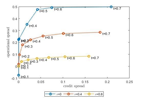
In what follows, we plot the firm’s credit spread against its operational spread, i.e., the
markup p − K 0 (I + i). Proposition 3.3 is confirmed in Figure 2: When the firm chooses
optimal hedging policy given the debt level F , the credit spread and operational spread are
positively correlated. This positive relationship is stronger when the firm is more financially
constrained, i.e., its pledgeability τ is lower. This is consistent with the novel implication of
our model: when the firm’s credit spread is higher, the financially constrained firm cuts the
operational hedging activity by a larger extent to save more cash at date-0, hoping to avoid
financial default given the more likely cash shortfall at date-1.
[Figure 2 HERE]
4.2 Endogenous F
Next, we examine the firm’s optimal debt policy, i.e., how the firm chooses the optimal
debt level F that matures in the interim, knowing that it will always choose an operational
hedging policy that maximizes the equity value given the existing debt level. To introduce
the benefit of debt to firm value, we assume that the firm enjoys a tax deduction for debt
28payments. Assuming t is the corporate tax rate, we can write firm value as:
E+D =
Z ∞
(1 − t) [x0 − K(I + i) + x̄1 + u + p ((1 − δ(u))I + i) + x2 ] g(u)du − λx2 G(uO )
0
| {z }
unlevered firm value
Z uF
− (1 − t) (1 − τ )p ((1 − δ(u))I + i) g(u)du + x2 G(uF ) − λx2 G (min{uO , uF })
0
| {z }
expected net bankruptcy cost
+ tF [1 − G(uF )] (4.1)
| {z }
tax benefit
As shown in the first term of Equation (4.1), debt level F creates a real inefficiency in
the sense that the optimal operational hedging policy in the presence of F deviates from
the first-best policy that maximizes the unlevered firm value. The second term is the
expected bankruptcy cost: If the firm declares bankruptcy, with probability G(uF ), eq-
uity holders lose the the expected unpledgeable income from supply contract delivery, as
well as franchise value x2 . Unlike the standard risky debt models (e.g., Acharya et al.,
2012), by declaring bankruptcy, equity holders avoid the cost of operational default, which
is λx2 G (min{uO , uF }). The last term captures the tax-shield benefit of debt.
Figure 3 presents the equilibrium debt policy and the equilibrium operational hedging
policy against τ ∈ [0, 0.8]. First, as shown in Figure 3a and Figure 3b, both the optimal
F and the optimal operational hedging policy i increase in τ . A fraction τ of operational
hedging amount i can be pledged to the creditors. As the pledgeability increases, operational
hedging policy resembles the cash savings policy in terms of lowering the probability of
financial default. Thus, the firm is willing to invest more in operational hedging activity.
Since the bankruptcy probability, and in turn the expected bankruptcy cost, is lower due to
higher pledgeability, the firm will also borrow more at date-0. Correspondingly, Figure 3c
29illustrates that the optimal debt policy and operational hedging policy mutually reinforce
each other as the pledgeability τ increases for most of τ range. Finally, when τ is higher,
the increase in equilibrium debt level and operational hedging level outweigh the debt risk
reduction from higher pledgeability. Consequently, the credit spread increases in τ , leading to
a negative relationship between credit spread and operational spread, as shown in Figure 3d.
[Figure 3 HERE]
Our next exercise characterizes the firm’s equilibrium debt and operational hedging po-
lices for various levels of corporate tax rate t. We vary t from 0.1 to 0.7. A higher tax
rate increases the marginal benefit of debt, thus the firm chooses a higher debt level F ,
as illustrated in Figure 4a. Figure 4b shows that the optimal operational hedging policy
decreases in the tax rate t. Taken together, Figure 4a and Figure 4b lead to a negative
relationship between the optimal debt policy F and operational hedging policy i, as shown
in Figure 4c. Moreover, in Figure 4c, the slope of the blue line (τ = 0 case) is steeper than
that of the red line (τ = 0.4 case), which is in turn steeper than that of the yellow line
(τ = 0.8 case), meaning that the negative relationship between debt policy and operational
hedging policy is stronger when the firm is more financially constrained, i.e., τ is lower. The
pattern is explained by the main message of the paper: when higher tax benefit induces the
firm to take on more debt, it reduces the operational hedging activity as it saves more cash
in order to reduce the financial default risk, especially when the firm lacks the ability to
pledge the income from supplier contract fulfillment to creditors. Lastly, the firm chooses
the optimal debt level that equalizes the marginal benefit (tax savings) and the marginal
cost (from financial and operational defaults). As the marginal benefit increases as a result
of a higher tax rate, the firm chooses a higher optimal F that also leads to a higher marginal
cost, which manifests itself in a higher credit spread and lower operational hedging. As a
30You can also read