BIS Working Papers Cyclical Fiscal Policy, Credit Constraints, and Industry Growth
←
→
Page content transcription
If your browser does not render page correctly, please read the page content below
BIS Working Papers
No 340
Cyclical Fiscal Policy, Credit
Constraints, and Industry
Growth
by Philippe Aghion, David Hemous and Enisse Kharroubi

Monetary and Economic Department

February 2011

JEL classification: E32, E62

Keywords: growth, financial dependence, fiscal policy,
countercyclicality
BIS Working Papers are written by members of the Monetary and Economic Department of
the Bank for International Settlements, and from time to time by other economists, and are
published by the Bank. The papers are on subjects of topical interest and are technical in
character. The views expressed in them are those of their authors and not necessarily the
views of the BIS.

Copies of publications are available from:
Bank for International Settlements
Communications
CH-4002 Basel, Switzerland

E-mail: publications@bis.org
Fax: +41 61 280 9100 and +41 61 280 8100
This publication is available on the BIS website (www.bis.org).

© Bank for International Settlements 2011. All rights reserved. Brief excerpts may be
  reproduced or translated provided the source is stated.

ISSN 1020-0959 (print)
ISBN 1682-7678 (online)
Cyclical Fiscal Policy, Credit Constraints, and Industry Growth∗

                            Philippe Aghion, David Hemous, Enisse Kharroubi

                                                   February 23, 2011

                                                          Abstract

          This paper analyzes the impact of cyclical fiscal policy on industry growth. Using Rajan and Zingales’

      (1998) difference-in-difference methodology on a panel data sample of manufacturing industries across

      15 OECD countries over the period 1980-2005, we show that industries with relatively heavier reliance

      on external finance or lower asset tangibility tend to grow faster (both in terms of value added and of

      labor productivity growth) in countries which implement more countercyclical fiscal policies.

      Keywords: growth, financial dependence, fiscal policy, countercyclicality

      JEL Classification: E32, E62

   ∗ We thank Marios Angeletos, Roel Beetsma, Claudio Borio, Olivier Blanchard, Andrea Caggese, Olivier Jeanne, Leonardo

Gambacorta, Ashoka Mody, Philippe Moutot, and seminar participants at the ASSA meetings in Atlanta, the Bank for Inter-
national Settlements, the Banque de France, the Brookings Institution, CEPR-ESSIM, CREI, ECFIN, the European Central
Bank, the IMF, MIT, NBER Summer Institute and the Paris School of Economics for helpful comments and suggestions. The
views expressed here are those of the authors and do not necessarily reflect the views of the Bank for International Settlements,
the Banque de France or the EuroSystem. Philippe Aghion, Harvard University, paghion@fas.harvard.edu; David Hemous,
Harvard University, hemous@fas.harvard.edu; Enisse Kharroubi, Bank for International Settlements, enisse.kharroubi@bis.org

                                                               1
1 Introduction
Standard macroeconomic textbooks generally comprise two largely separate parts: the analysis of long-run
growth, which is linked to structural characteristics of the economy (education, R&D, openness to trade,
financial development) and short-term analysis, which emphasizes the short-term effects of productivity or
demand shocks and the effects of macroeconomic policies (fiscal and/or monetary) aimed at stabilizing the
economy. Yet the view that short-run stabilization policies should have no significant impact on long-run
growth has been challenged by several empirical papers, notably Ramey and Ramey (1995), who find a
negative correlation in cross-country regression between volatility and long-run growth.1 More recently,
using a Schumpeterian growth framework, Aghion et al (2005) have argued that higher macroeconomic
volatility affects the composition of firms’ investments and in particular pushes towards more procyclical
R&D investments in firms that are more credit-constrained.
This paper takes a further step by analyzing the effect of stabilizing fiscal policy on (industry) growth,
and how this effect depends upon the financial constraints faced by the industry.
In the first part of the paper we sketch an illustrative model to rationalize our empirical strategy and
predictions. In our model, which is a toy version of that developed by Aghion et al (2005), firms choose to
direct their investments either towards short-run projects that do not increase the stock of knowledge in the
economy, or towards productivity-enhancing long-term projects (e.g, R&D investments). The completion
of long-term innovative projects is in turn subject to a liquidity risk: namely, such projects can only be
implemented if the firm overcomes a liquidity shock that may occur during the interim period. A reduction
in aggregate volatility increases profits from short-term projects in the bad state of the world, and reduces
them in the good state of the world. Absent credit constraints, this decreases the incentive to invest in
long-term growth-enhancing projects in the bad state, whereas it increases long-term investment incentives
in the good state (the literature refers to this as the opportunity cost effect of volatility), so that the overall
effect on average R&D and growth is ambiguous. However, if credit constraints bind in the low state of
1 Additionalevidence can be found in Bruno (1993) on inflation and growth, Gavin and Hausman (1996) for Latin American
countries, or, more recently, Imbs (2007).
2the world only, the negative impact of the opportunity cost effect on the amount of investment undertaken
in the bad state of the world is compensated by the increase in the likelihood that long-term projects will
survive liquidity shocks in the bad state. Moreover, reducing volatility will increase the likelihood that
long-term projects will survive liquidity shocks in the bad state. We thus predict that by reducing aggregate
volatility a countercyclical fiscal policy should have a positive impact on R&D and on the growth rate of
more credit-constrained industries.2
In the second part of the paper, we take our prediction to the data. Departing from the existing empirical
literature on volatility and growth, which relies mainly on cross-country regressions, we follow here the
methodology developed in the seminal paper by Rajan and Zingales (1998). We use cross-industry/cross-
country panel data on a sample of 15 OECD countries over the period 1980-2005, to test whether industry
growth is significantly affected by the interaction between fiscal policy countercyclicality (computed for each
country as the fiscal balance to GDP sensitivity to the output gap) and external financial dependence or asset
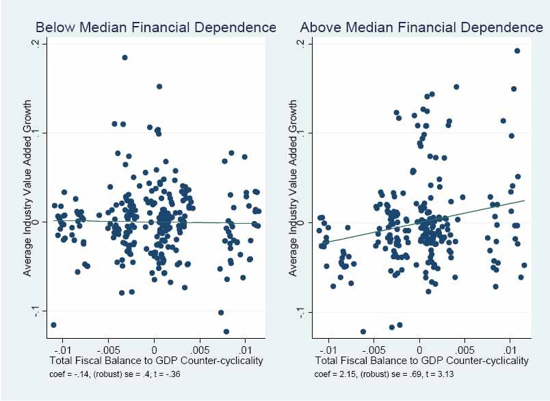
tangibility (measured for the corresponding industry in the US). Figure 1 summarizes our main findings:
it plots value added growth for a set of manufacturing industries as a function of total fiscal balance to
GDP countercyclicality, controlling for initial industry size. The left-hand panel in Figure 1 depicts this
relationship for industries with below-median levels of financial dependence, whereas the right-hand panel
plots this relationship for industries with above-median levels of financial dependence.3 We see that a more
countercyclical fiscal policy has virtually no effect on value added growth for industries with below-median
levels of financial dependence, i.e. that face milder credit constraints.
2 See Aghion et al (2009) for firm-level evidence of an asymmetric effect of credit constraints on R&D over firm’s business
cycle.
3 More precisely, the estimated equation is g
= + fp − log y + , where g is the average growth in industry in
country , fp measures fiscal policy countercyclicality (here, the output gap sensitivity of total fiscal balance to GDP), y is
the initial share of industry in country in total manufacturing valued added in country . Parameters for estimation are ,
and , while is a residual. This equation is estimated separately for industries with below-median financial dependence and
with above-median financial dependence. For the former, the estimated coefficient is −14 and is insignificant at standard
confidence levels. For the latter, the estimated coefficient is 215 and is significant at standard confidence levels (5% level).
3Figure 1
On the contrary, a more countercyclical fiscal policy has a positive and significant impact on real value added
growth for industries with above median-levels of financial dependence, i.e. with tighter credit constraints.
Using the same methodology, a similar result can be derived decomposing the sample between industries
with below-median asset tangibility and with above-median asset tangibility: industry growth and total fiscal
balance to GDP countercyclicality are positively ans significantly associated for industries whose assets are
relatively intangible (i.e. industries with below-median asset tangibility). However, there is no significant
relationship between total fiscal balance to GDP countercyclicality and industry growth for industries whose
assets are relatively tangible (i.e. industries with above-median asset tangibility).
The empirical analysis in this paper aims at establishing the robustness of these findings. Our empirical
results can be summarized as follows. First, fiscal policy countercyclicality - measured as the sensitivity of
a country’s total or primary fiscal balance (relative to GDP) to time variations in its output gap - has a
4disproportionate positive significant and robust impact on industry growth, the higher the extent to which
the corresponding industry in the US relies on external finance, or the lower the asset tangibility of the
corresponding sector in the US. This result holds whether industry growth is measured by real value added
growth or by labour productivity growth. It also holds for industry-level R&D expenditures. Moreover, this
interaction between financial dependence and countercyclical fiscal policy is stronger in recessions than in
booms, which in turn echoes the asymmetry between good and bad states emphasized in the model. Yet,
the ability to tighten fiscal policy in booms remains a significant determinant of growth when interacted
with industry external financial dependence. Besides, two factors should be borne in mind when interpreting
this last result. First, sustainability issues are not directly addressed and second recent experience shows
that credit and asset price booms that precede financial distress tend to flatter fiscal accounts, thereby
underestimating the cyclical component. All this puts a premium on the need to be prudent in good times.
Using the regression coefficients, one can assess the magnitude of the corresponding difference-in-difference
effect: that is, how much extra growth is generated when fiscal policy countercyclicality and external financial
dependence move from the 25th to the 75th percentile? The figures happen to be relatively large, especially
when compared to the equivalent figures in Rajan and Zingales (1998). This, in turn, suggests that the effect
of a more countercyclical fiscal policy in more financially constrained industries is economically significant.
Second, we show that our baseline result is robust to: (i) a whole set of alternative measures of fiscal
policy cyclicality; (ii) adding control variables such as financial development, inflation, and average fiscal
balance interacted with the industry level variables (external financial dependence or asset tangibility); (iii)
taking into account the uncertainty around fiscal policy cyclicality estimates (iv) instrumenting fiscal policy
cyclicality with economic, legal and political variables.4
What do we gain by moving from cross-country to cross-industry analysis? A pure cross-country analysis
raises at least three issues. First, the cyclicality of (fiscal) policy is typically captured by a unique time-
invariant parameter which only varies across countries. As a result, standard cross-country panel regression
cannot be used to assess the effect of the cyclical pattern of fiscal policy on growth inasmuch as the former is
4 For the sake of brevity, estimations dealing with issues (i) and (ii) are not presented in the paper, but are available upon
request.
5perfectly collinear to the fixed effect that is traditionally introduced to control for unobserved cross-country
heterogeneity.5 Second, the causality issue (does a positive correlation between fiscal policy countercyclicality
and growth reflect the effect of fiscal policy cyclicality on growth or the effect of growth on the cyclical pattern
of fiscal policy) cannot be properly addressed while keeping the analysis at a purely macroeconomic level.6
A final concern is identification: a cross-country panel regression, particularly one which is restricted to a
small cross-country sample, is unlikely to be robust to the inclusion of additional control variables reflecting
alternative stories. Thus, even if cross-country panel regressions point to correlations between the cyclical
pattern of fiscal policy and growth, the channel through which this correlation works is not likely to be well
identified by a pure country-level analysis.
Our industry-level analysis helps us address these concerns. First, even though we estimate the coun-
tercyclicality of fiscal policy at the country level with a time-invariant coefficient, which implies that fiscal
policy countercyclicality in each country is collinear to that country’s fixed effect, the interaction between
the country-level measure of countercyclicality and the industry level variable is not. Second, by working at
cross-industry level we have enough observations that our results withstand the introduction of country and
industry fixed effects plus a whole set of structural variables as additional controls. Finally, to the extent
that macroeconomic policy should affect industry level growth whereas the opposite - industry level growth
affecting macroeconomic policy- is less likely to hold, finding a positive and significant interaction coefficient
in the growth regressions is more likely to reflect a causal impact of the cyclical pattern of fiscal policy
on growth.7 However, there is a downside to the industry-level investigation: namely, our cross-sectoral
differences-in-differences analysis has little to say about the aggregate magnitude of the macroeconomic
growth gain/loss induced by different patterns of cyclicality in fiscal policy.8
5 To overcome this problem, Aghion and Marinescu (2007) introduce time-varying estimates of fiscal policy cyclicality. While
this helps control for unobserved heterogeneity, it comes at the cost of losing precision in the estimates of fiscal policy cyclicality.
6 One particular reason for this is that fiscal policy cyclicality is used in growth regressions as a right-hand side variable while
the estimation of time-varying fiscal policy cyclicality requires using the full data sample. See Aghion and Marinescu (2007).
7 Fiscal policy cyclicality could be endogenous to the industry-level composition of total output if, for example, industries
that benefit more from fiscal policy countercyclicality do lobby more for countercyclical fiscal policy. However, to the extent
that there are decreasing returns to scale (which is likely to be the case in the manufacturing industries featured in our empirical
analysis), this would rather imply a downward bias in our estimates of the positive impact of fiscal policy countercyclicality
on growth. Hence, controlling for this possible source of endogeneity would only reinforce our conclusions by reducing this
downward bias.
8 The fact that we focus on manufacturing industries, and leave out the service sector makes it even harder to use our results
to derive more aggregate numerical conclusions.
6Our analysis contributes to at least three ongoing debates among macroeconomists: 1) is there a (causal)
link between volatility and growth?; 2) what is the optimal design of intertemporal fiscal policy?; and 3)
what are the effects of a countercyclical fiscal stimulus on aggregate output? Acemoglu and Zilibotti (1997)
stress that the correlation between long-term growth and volatility is not entirely causal pointing to low
financial development as a factor that could both reduce long-run growth and increase the volatility of the
economy. More recently, Acemoglu et al (2003) and Easterly (2005) hold that both high volatility and
low long-run growth arise not directly from policy decisions but rather from bad institutions. However,
fiscal policy cyclicality varies significantly even among OECD countries (Lane, 2003) which share similar
institutions. And our own finding of significant correlations between growth and countercyclical fiscal policy
in a sample of OECD countries also speaks to the importance of cyclical fiscal policy, over and above the
effect of more structural variables. As mentioned previously, Aghion et al (2005) defend the view that higher
volatility should induce lower growth by discouraging long-term growth-enhancing investments, particularly
in more credit-constrained firms. Aghion et al (2009) build on that insight when analyzing the relationship
between long-run growth and the choice of exchange-rate regime.9
The case for a countercyclical fiscal policy was most forcefully made by Barro (1979): it helps smooth
out intertemporal consumption when production is affected by exogenous shocks, thereby improving welfare.
Another justification for countercyclical fiscal policy stems from a more Keynesian view of the cycle: namely,
to the extent that a recession corresponds to an increase in the inefficiency of the economy, appropriate fiscal
or monetary policy that raises aggregate demand can bring the economy closer to the efficient level of
production (see Galí, Gertler, López-Salido, 2007).10 The effect of fiscal policy in our model is different:
fiscal policy affects growth through a market-size effect: e.g. by increasing expenditures, the government
can induce firms to devote more investment to long-term projects, as innovations will then pay out more.11
Finally, an extended literature looks at the - short-run - output response to an exogenous increase in
9 See Aghion and Banerjee (2005) and Aghion and Howitt (2009, ch14) for more complete literature reviews on the link
between volatility and long-run growth.
1 0 Consequently, government purchases need to remain above the level implied by the optimal provision of public good, as
their role is dual: providing a public good, and increasing the efficiency in the economy (Galí, 2005).
1 1 In Barro (1990)’s AK model, however, growth decreases with utility-type government expenditures and increases only
initially with productive government expenditures.
7government spending or to a tax cut. Importantly in these papers, GDP is usually detrended, so that all
long-run effects are shut down. Although most economists would agree that a fiscal shock should increase
short-run output, there is no consensus on the magnitude of the effect.12 In particular, papers that introduce
rational expectations and long-run wealth effects will typically predict a lower value of the multiplier (based
on the idea that consumers anticipate that an increase in government spending today is likely to result in
an increase in taxes tomorrow).13 We move beyond this debate by looking only at the long-run effect of a
more countercyclical fiscal policy: even if the short-run effect of a more countercyclical policy were more in
line with the prediction of low multipliers, our results point to economically significant long-run effects.
The remaining part of the paper is organized as follows. Section 2 presents the model which helps us
organize our thoughts and formulate our main prediction. Section 3 describes the econometric methodology
and the data sources used in our estimations. Section 4 presents our empirical results and discusses their
robustness. Section 5 concludes.
2 Cyclical fiscal policy and growth: an illustrative model
In this section we develop a simple model to rationalize our following empirical findings, namely that coun-
tercyclical fiscal policy is more growth- and R&D-enhancing in sectors that are more credit-constrained, the
effect being driven by what happens in the low states of the world where credit constraints are more binding.
1 2 Skeptical views on the importance of the effect of fiscal shocks include Andrew Mountford and Harald Uhlig (2008) or
Roberto Perotti (2005). On the other hand, Antonio Fatás and Ilian Mihov (2001b) find that an increase in government
spending (especially government wage expenditures increase) induces increases in consumption and employment. All the above
mentioned papers use VAR analysis, and Olivier Blanchard and Roberto Perotti (2002) use a mixed VAR - event study
approach to show that both, increases in government spending and tax cuts have a positive effect on GDP; they also find - like
Alberto Alesina et al (2002) - that fiscal policy shocks have a negative effect on investment; note that this does not contradict
our theory which points at investments being directed towards more productivity enhancing projects as the channel whereby
long-run growth is enhanced by a more countercyclical fiscal policy.
Somewhat closer to the analysis in this paper, Athanasios Tagkalakis (2008) shows on a panel of 19 OECD countries from 1970
to 2002 that the effects of fiscal policy changes on private consumption is higher in recessions than in expansions. Interestingly,
they explain this phenomenon by the presence of more liquidity constrained consumers in recessions, and show that the effect
is more pronounced in countries characterized by less developed consumer credit markets.
1 3 For example John F. Cogan et al (2009) use the Frank Smets and Rafael Wouters (2007) model and compute the effect of
a permanent increase by 1% of GDP of government expenditures as of 2009: by 2011 Q4, they find that the increase in GDP is
only equal to 0.44%, whereas Christina D. Romer and Jared Bernstein (2009) find a 1.57% increase. Finally, based on narrative
records, Christina D. Romer and David H. Romer (2007) find that - exogenous - tax increases are highly contractionary.
82.1 Basic setup
The environment The model builds on Aghion et al (2005). We consider a discrete time model of an
economy populated by a continuum of two-periods lived risk neutral entrepreneurs (firms).
Each firm starts out with a positive amount of wealth = , where denotes the accumulated
knowledge at the beginning of the current period , and denotes the firm’s knowledge adjusted wealth.
Initial wealth can be invested in two types of projects: a short term investment project which generates
output in the current period and a long term innovation project which, when successful, generates production
with higher productivity next period. The short term investment project may involve maintaining existing
equipment, expanding a business using the same kind of technology and equipment, or increasing marketing
expenses. The long term project may consist in learning a new skill, learning about a new technology,
or investing in R&D. Investing in the long term project increases the stock of knowledge available in the
economy next period, whereas investing in the short term project does not contribute to knowledge growth.
Both, short term and long term profits are proportional to market demand (see Daron Acemoglu and Joshua
Linn, 2004).14
More specifically, by investing capital = in the short term project at time , where denotes
the knowledge adjusted short-run capital investment, a firm generates short-run profits
Π1 ( ) = 1 ( )
where is an aggregate shock at time and 1 ( ) is the normalized short-run profit, 1 being increasing
and weakly concave. follows a Markovian process. We assume that ∈ { } with and
¡ ¯ ¢
Pr +1 = ¯ = = 12 for ∈ { }.15
Now, consider firms’ long term investments. Following Aghion et al (2005), we shall assume that after the
1 4 In this set-up, short- and long-term investments may increase the mark-ups that firms can charge, but they have no effect
on total production which is pinned down by the market size variable detailed below.
1 5 We can easily extend our analysis to the case of a persistent aggregate shock, with
Pr +1 = = = ≥ 12
.
9R&D investment = has been incurred, where denotes the knowledge-adjusted long-term innovative
investment, the firm faces an idiosyncratic liquidity shock = drawn in a uniform distribution over
[0; ]. The firm reaps the profits of its long-term investments (and the liquidity shock including the interest
payment) if and only if it is able to pay for the liquidity cost , such long term profits write as
¡ ¢
Π2 +1 = +1 2 ( )
where 2 ( ) is the normalized long-term profit in present value terms, 2 being increasing and concave.
Thus here we implicitly assume that the liquidity shock is either paid and then recouped ex post including
interest payments on it, or not paid at all.
While liquidity shocks are private information and hence cannot be diversified, firms can still borrow
once the liquidity shock is realized. Following Aghion et al (2005), a firm cannot borrow more than − 1
times their current cash flow in order to overcome the liquidity shock.16 17 Long-term investments survive
the liquidity shock with probability
( ) = Pr( ≤ 1 ( ))
The parameter can be interpreted as a proxy for the tangibility of the firm’ assets: more tangible assets
being typically associated with lower monitoring costs for potential creditors, and therefore to a higher value
of the credit multiplier . Similarly the parameter can be interpreted as the extent to which the firm
depends upon external finance: the higher the less likely the firm will be able to cover its liquidity shock
using only its retained earnings 1 ( ).
Knowledge growth results from investments in long-term projects that overcome the liquidity shock.
1 6 This type of borrowing constraint can be based on ex post moral hazard considerations. See Philippe Aghion, Abhijit
Banerjee and Thomas Piketty (1999). Note that the existence of borrowing constraints also prevents firms from achieving
insurance against idiosyncratic liquidity shocks.
1 7 Following Aghion, Banerjee and Piketty (1999) or Aghion et al (2005), we take to be constant over time. Alternative
formulations, for example Bengt Holmstrom and Jean Tirole (1995) based on ex ante moral hazard, would generate a credit
multiplier which is negatively correlated with the interest rate, and therefore typically procyclical. A procyclical would only
reinforce the optimality of countercyclical fiscal policy established later in this section.
10More formally, the growth rate +1 between period and period + 1 is given by:18
+1 −
+1 = = ( ) (1)
Timing of events The overall timing of events is as follows:
(i) The state of nature in period happens; new firms make their investment decisions based on current
government policy and the policy they anticipate in the following period,
(ii) Short-term investments and liquidity shocks are realized. A capital market opens. Firms that have
accumulated enough wealth to overcome their liquidity shock lend to those that have not,
(iii) Firms that have overcome their idiosyncratic liquidity shocks in period realize their long term invest-
ment at the beginning of period + 1.
2.2 A firm’s maximization problem
In this subsection we analyze firms’ optimal investment decisions. Given that firms are ex ante identical,
there exists a symmetric equilibrium where all firms make the same investment decisions, and we focus our
attention on this particular equilibrium.19 Once the state of nature at time is realized, a representative
firm chooses investments to maximize its expected present value, that is the sum of its current profits and
of its expected future revenues; more formally it chooses investments ( ) to
¡ ¡ ¢ ¢
max
Π1 ( ) + Π2 +1 |
;
subject to: + ≤
1 8 Alternatively, the growth rate could be proportional to the profits realized from long-term investments instead of being
2
proportional to long-term investments (note that if 2 were to represent the probability of discovering a new technology, this
would be a natural assumption to make).
1 9 Given that all firms start out with same initial wealth = there is no borrowing and lending in equilibrium at
the beginning of a period. However, once the idiosyncratic liquidity shocks are realized, firms with low liquidity shocks will
typically lend to firms facing higher liquidity shocks.
11which simplifies to:
max
1 ( ) + Pr ( ≤ 1 ( )) 2 ( )
;
subject to: + ≤
¡ ¢
where = +1 | = = 12 + 12
We will consider the effects on the expected growth rate of reducing the variance of +1 conditional on
=
The first term 1 ( ) corresponds to knowledge adjusted profits derived from short term investments.
The second term which represents the expected profits derived from long term investments is the product of
three items. The first item Pr ( ≤ 1 ( )) is the probability that long term investments go through the
liquidity shock. represents the expected aggregate shock at time + 1. The last term 2 ( ) represents
the normalized long-term profit.
2.3 Analysis
Assume that credit constraint does not bind in the good state, = . Then the entrepreneur’s problem
writes as
max 1 ( − ) + 2 ( )
∗
Assuming an interior solution, the optimal long term investment = satisfies
02 (
∗
) = 01 ( −
∗
) (2)
In particular, a reduction in the variance of +1 keeping constant, decreases and therefore increases
∗
optimal long term investment This is commonly referred to as the opportunity cost effect.
Now we turn to the low state = First, if the credit constraint does not bind in that state, then
∗
the optimal R&D investment = is subject to the same opportunity cost effect, with
∗ ∗
02 ( ) = 01 ( − ) (3)
12∗ 20
and therefore a reduction in aggregate volatility which amounts to increasing results in decreasing .
Now, if the credit constraint binds in the low state, the entrepreneurs’s problem writes as
h i
max 1 ( − ) + 1 ( − ) 2 ( )
∗
Assuming an interior solution,21 the optimal long term investment = satisfies
³ ´
∙ ¸ 0 − ∗
∗ ∗ 1
02 ( ) = 2 ( )+ ³ ´ (4)
1 − ∗
∗
In particular, a reduction in volatility has no effect on : what happens here is that the opportunity
cost effect is exactly offset by a liquidity effect, namely the fact that increasing increases the probability
that the long-term project survives; that these two effects exactly compensate each other is an artifact of
the uniform distribution assumption on 22
∗
Moreover, note that in this case the optimal long-term investment in the low state is larger the
lower the and/or the higher the . In other words, when credit constraints are relaxed, the profitability of
long-term investments increases which in turn encourages more long-term investment.
2.4 Growth effect of government spending countercyclicality
Recall that the growth rate +1 between period and period + 1 is given by (1). Therefore, when the
credit constraint never binds, the expected growth rate +1 writes as
1 ∗ 1 ∗
+1 = + (5)
2 2
2 0 Logically, because of the opportunity cost effect, ∗ ∗ , so that the credit constraint is more likely to bind in the
low state of the world than in the high state.
2 1 We deal with the non-interior solution case in the Appendix A.
2 2 If the distribution of shocks is not uniformly distributed then current aggregate shock will typically affect the investment
in long-term projects also in the low state of the world. In particular, one can show that in the case of a Pareto distribution
with parameter smaller than 1, an increase in will increase investment in long-term projects.
13In particular a reduction in aggregate volatility can either raise or reduce average growth: on the one hand a
lower decreases the opportunity cost effect which increases R&D investment; on the other hand a higher
increases the opportunity cost effect which reduces R&D investment.
When the credit constraint binds only in the low state of the world, the expected growth rate +1
between periods and + 1 is simply equal to:
³ ´
∗
1 1 − ∗ 1 ∗
+1 = + (6)
2 2
It then follows that a reduction in aggregate volatility increases average growth: first, a lower decreases
the opportunity cost effect which increases R&D investment; second, a higher raises the number of R&D
projects that survive the liquidity shock without affecting the aggregate R&D effort.
This establishes:
Proposition 1 A small reduction in aggregate volatility has an ambiguous effect on the average growth rate
if the credit constraint never binds, whereas it has a positive effect on the aggregate growth rate if it binds
only in the low state.
An important implication of this proposition is that a countercyclical fiscal policy which would reduce
the volatility of the aggregate shocks faced by firms, will be more growth-enhancing for firms that face
tighter credit constraints, when credit constraints are (more) binding in the low states of the world.23 This
is because, in the low state of nature, a more counter-cyclical fiscal policy tends to raise successful R&D
investment for firms whose credit constraint is binding while it tends to reduce R&D investment for firms
whose credit constraint is not binding.
To conclude this section, note that if credit constraints were to bind in both states of the world, then a
reduction in aggregate volatility would not affect expected growth in this set-up with = 12. Yet, it might
2 3 The difference between the expected growth rate of a sector where the credit constraint binds in the low state, and one
where it never binds writes simply as:
∗
1 1 − ∗ 1 ∗
−
2 2
∗ ∗
As is independent of and decreases in , this term is unambiguously positive.
14actually result in a higher expected number of surviving long-term projects, i.e. in higher growth, as more
long term investment would be undertaken in the high state, if there is positive persistence in the aggregate
shock. However, our empirical analysis suggests that this "gambling for resurrection" effect is dominated in
the data.
3 Econometric methodology and data
We investigate whether differences in fiscal policy cyclicality across countries and in financial constraints
across industries can account for cross-country cross industry growth differences. To do so, we consider
an empirical specification in which our dependent variable is the average annual growth rate of labour
productivity or real value added in industry in country for a given period of time, say [; + ]. Labour
productivity is defined as the ratio of real value added to total employment.24 On the right hand side
(henceforth, RHS), we introduce our variable of interest (sc )×(fp ), namely the interaction between industry
’s specific characteristic (sc ) (external financial dependence or asset tangibility), and the degree of (counter-
) cyclicality of fiscal policy (fp ) in country over the period [ + ]. Moreover, we control for initial
conditions by including the term log y as an additional regressor on the RHS of the estimation equation.
When labour productivity (resp. value added) growth is the dependent variable, y represents the beginning
of period ratio of labour productivity (resp. value added) in industry in country to total manufacturing
labor productivity (resp. total manufacturing real value added) in country . Finally, we introduce a full set
of industry and country fixed effects { ; } to control for unobserved heterogeneity across industries and
across countries. Letting denote the error term, our main estimation equation -which we will also refer
to as the second stage regression- can then be expressed as:
g = + + (sc ) × (fp ) − log y + (7)
2 4 Although we also have access to industry level data on hours worked, we prefer to focus on productivity per worker and
not productivity per hour as measurement error is more likely to affect the latter than the former.
15Following Rajan and Zingales (1998) we measure industry specific characteristics using firm level data in
the US. External financial dependence is measured as the average across all firms in a given industry of
the ratio of capital expenditures minus current cash flow to total capital expenditures. Asset tangibility is
measured as the average across all firms in a given industry of the ratio of the value of net property, plant
and equipment to total assets. This methodology is predicated on the assumptions that: (i) differences in
financial dependence/asset tangibility across industries are largely driven by differences in technology; (ii)
technological differences persist over time across countries; (iii) countries are relatively similar in terms of
the overall institutional environment faced by firms. Under those three assumptions, the US based industry-
specific measure is likely to be a valid interactor for industries in countries other than the US.25 Now, there are
good reasons to believe that these assumptions are satisfied particularly if we restrict the empirical analysis
to a sample of OECD countries. For example, if pharmaceuticals require proportionally more external
finance than textiles in the US, this is likely to be the case in other OECD countries. Moreover, since little
convergence has occurred among OECD countries over the past twenty years, cross-country differences are
likely to persist over time. Finally, to the extent that the US are more financially developed than other
countries worldwide, US based measures of financial dependence as well as asset tangibility are likely to
provide the least noisy measures of industry level financial dependence or asset tangibility.
We next focus attention on how to measure fiscal policy cyclicality over the time interval [ + ] i.e.
how to construct the RHS variable (fp ). Given that fiscal policy cyclicality cannot be observed, we need an
"auxiliary" equation -which we will also refer to as the first stage regression- to infer fiscal policy cyclicality
for each country of the sample. Our approach is to estimate fiscal policy cyclicality as the marginal change
in fiscal policy stemming from a given change in the domestic output gap. Thus we use country-level data
over the period [; + ] to estimate the following country-by-country "auxiliary" equation:
fb = + fp z + (8)
2 5 Note however that this measure is unlikely to be valid for the US as it likely reflects the equilibrium of supply and demand
for capital in the US and therefore is endogenous.
16where: (i) ∈ [; + ] ; (ii) fb is a measure of fiscal policy in country in year : for example total fiscal
balance to GDP; (iii) z measures the output gap in country in year , that is the percentage difference
between actual and potential GDP, and therefore represents the country’s current position in the cycle; (iv)
is a constant and is an error term. Equation (8) is estimated separately for each country in our
sample. For example, if the LHS of (8) is the ratio of fiscal balance to GDP, a positive (resp. negative)
regression coefficient (fp ) reflects a countercyclical (resp. pro-cyclical) fiscal policy as the country’s fiscal
balance improves (resp. deteriorates) in upturns. Moreover, as a robustness check, we consider the case
where fiscal policy indicators in regression (8) are measured as a ratio to potential and not current GDP.
This alternative specification helps make sure that the cyclicality parameter (fp ) captures changes in the
numerator of the LHS variable -related to fiscal policy- rather than in the denominator -related to cyclical
variations in output-.26 Furthermore more elaborated fiscal policy specifications can also be considered. In
particular, following Jordi Galí et al (2003), a debt stabilization motive as well as a control for fiscal policy
persistence can be included on the RHS. Thus, letting b denote the ratio of public debt to potential GDP
¡ ¢
in country in year , we could estimate fiscal policy cyclicality fp2 over the period [; + ] using the
modified "auxiliary" equation:
fb = + fb −1 + fp2 z + b −1 + (9)
where z is as previously the output gap in country in year , fb −1 is the fiscal policy indicator in
country in year − 1 and is an error term.
Following Rajan and Zingales (1998), when estimating our second stage regression (7) we rely on a simple
OLS procedure, correcting for heteroskedasticity bias whenever needed, without worrying much further about
endogeneity issues. In particular, the interaction term between industry specific characteristics and fiscal
policy cyclicality is likely to be largely exogenous to the LHS variable, be it industry labour productivity
2 6 When data is available, we also measure fiscal policy using cyclically adjusted variables. In this case, the cyclicality of fiscal
policy results more directly from discretionary policy. Put differently, cyclicality stemming from automatic stabilizers is purged
out. Unreported results -available upon request- are very similar to the case where fiscal policy indicators are not cyclically
adjusted.
17or value added growth. First, our external financial dependence variable pertains to industries in the US
while the growth variables on the LHS involves other countries than the US. Hence reverse causality whereby
industry growth outside the US could affect external financial dependence or asset tangibility of industries
in the US, seems quite implausible. Second, fiscal policy cyclicality is measured at a macro level whereas
the LHS growth variable is measured at industry level, which again reduces the scope for reverse causality
as long as each individual industry represents a small share of total output in the domestic economy. Yet,
as an additional test that our results are not driven by endogeneity considerations, we produce additional
regressions where we instrument for fiscal policy cyclicality.27
Our data sample focuses on 15 industrialized OECD countries plus the US. In particular, we do not include
Central and Eastern European countries and other emerging market economies. Industry-level data for this
country sample are available for the period 1980-2005 while R&D data are only available for the period 1988-
2005.28 Our data come from four different sources. Industry level real value added and labour productivity
data are drawn from the EU KLEMS dataset while Industry level R&D data is drawn from OECD STAN
database.29 The primary source of data for measuring industry financial dependence, is Compustat which
gathers balance sheets and income statements for US listed firms. We draw on Rajan and Zingales (1998)
and Claudio Raddatz (2006) to compute the industry level indicators for financial dependence.30 We draw
on Matías Braun and Borja Larrain (2005) to compute industry level indicators for asset tangibility. Finally,
macroeconomic fiscal and other control variables are drawn from the OECD Economic Outlook dataset and
from the World Bank Financial Development and Structure database.31
2 7 Our IV tables below show a large degree of similarity between OLS and IV estimations, thereby confirming that our basic
empirical strategy properly addresses the endogeneity issue, even though it uses OLS estimations.
2 8 We present here the empirical results related to the 1980-2005 period. Estimations on sub-samples with shorter time span
are available upon request. Cf. Appendix B for more details on the data and country sample.
2 9 These data are available respectively from: http://www.euklems.net/data/08i/all_countries_08I.txt and
http://stats.oecd.org/Index.aspx
3 0 Rajan and Zingales data is accessible at: http://faculty.chicagogsb.edu/luigi.zingales/research/financing.htm
3 1 The OECD Economic Outlook dataset is accessible at: http://titania.sourceoecd.org. The World Bank Financial Develop-
ment and Structure database is accessible at: http://siteresources.worldbank.org
184 Results
4.1 The first stage estimation
We first focus on first stage regressions which deliver estimates for fiscal policy cyclicality. The first histogram
(figure 2) provides the country by country estimates for fiscal policy cyclicality when the dependent variable
in equation (8) is total fiscal balance to potential GDP as well as the estimated confidence interval at the
10 percent level for each country.32 According to these estimates, the most counter-cyclical countries of our
sample are Sweden and Denmark. In Sweden, total fiscal balance to potential GDP tends to increase by 1.7
percentage point in response to a 1 percentage point increase in the domestic output gap. In Denmark, the
corresponding increase is of almost 1.5 percentage point. In these two countries, the government is more
likely to run a surplus when the economy experiences a boom (i.e. a positive output gap) and is more
likely to run a deficit when the economy experiences a bust (i.e. a negative output gap). Conversely, the
least counter-cyclical countries -put differently, the most pro-cyclical countries- of our sample are Greece and
Italy. In these two countries, the sensitivity to the domestic output gap of the ratio of total fiscal balance
to potential GDP is negative: the government runs a larger surplus or a lower deficit, when the output gap
decreases, i.e. when the economy deteriorates. Note however that for both countries (Greece and Italy), the
estimated coefficient is not significant since the hypothesis that it is equal to zero cannot be rejected at the
10 percent level given the confidence bands. The second histogram (figure 3) provides the country by country
estimates for fiscal policy cyclicality when the dependent variable in equation (8) is primary fiscal balance to
potential GDP. The difference between total and primary fiscal balance is that the latter excludes interest
payments to or from the government. This histogram is similar to the first one. In particular, Denmark and
Sweden remain the most counter-cyclical countries of our sample while Greece and Italy are still the most
pro-cyclical countries. A key difference between the two histograms however is that primary fiscal balance
to potential GDP ratio is significantly pro-cyclical in Greece and Italy for the two latter countries whereas
the ratio of total fiscal balance to GDP is not.
3 2 The confidence interval at the 10% level is built as [ − 165; + 165] where and respectively denote the estimated
coefficient and standard error for fiscal policy cyclicality using equation (8).
19Next we look at bivariate correlations between fiscal policy cyclicality and macroeconomic variables.
Empirical evidence first shows that fiscal policy countercyclicality is positively associated with the size of
the government (figure 4). Indeed the correlation between total fiscal balance to GDP countercyclicality
and average total fiscal expenditures to GDP is positive and significant. However this correlation is only
marginally significant. When government size is captured by the ratio of average primary -rather than total-
fiscal expenditures to GDP, the correlation remains positive, and with much larger significance. Next we
investigate the correlation between fiscal countercyclicality and fiscal discipline (figure 5). Here, there is a
strong positive association between total fiscal balance to GDP countercyclicality and average total fiscal
balance to GDP. This means that countries which have run the largest average deficits have also run the
least counter-cyclical or the most pro-cyclical fiscal policies. Note however that this result does not hold
in the case of primary fiscal balance since then the correlation between primary fiscal balance to GDP
countercyclicality and average primary fiscal balance to GDP while still positive is not significant. Finally,
we look at the relationship between fiscal cyclicality and macroeconomic volatility (figure 6). Figure 6 shows
that there is a significantly negative correlation between fiscal countercyclicality and the volatility in labour
productivity growth. This result is not too surprising: a more counter-cyclical fiscal policy should have a
more dampening effect on aggregate volatility.
4.2 The second stage estimation
We first estimate our main regression equation (7), with real value added growth as LHS variable, using
financial dependence or asset tangibility as industry-specific interactors (table 1). Fiscal policy cyclicality
is estimated using alternatively the ratio of total or primary fiscal balance to actual or potential GDP as
LHS fiscal policy indicator in regression (8). The difference between these total and primary fiscal balance
is that the latter does not include net interest repayments to/from the government. The empirical results
show that real value added growth is significantly and positively (resp. negatively) correlated with the
interaction of external financial dependence (resp. asset tangibility) and fiscal policy countercyclicality: a
larger sensitivity to the output gap of total fiscal balance to GDP (actual or potential) raises industry real
20valued added growth the more so for industries with higher financial dependence or for industries with lower
asset tangibility.
The results are qualitatively similar when using primary fiscal balance: industries with larger financial
dependence or lower asset tangibility tend to benefit more from a more countercyclical fiscal policy in the
sense of a larger sensitivity of the primary fiscal balance to variations in the output gap. Estimated coefficients
are however smaller in absolute value when fiscal policy is measured through primary fiscal balance. This is
related to the fact that the cross-country dispersion in the cyclicality of primary fiscal balance is larger than
the cross-country dispersion in the cyclicality of total fiscal balance.
Three remarks are worth making at this point. First, the estimated coefficients are highly significant -in
spite of the relatively conservative standard errors estimates which we cluster at the country level-. Second,
the pairwise correlation between industry financial dependence and industry asset tangibility is around −06
which is significantly below −1. In other words, these two variables are far from being perfectly negatively
correlated, which in turn implies that the regressions with financial dependence as the industry specific
characteristic are not just mirroring regressions where asset tangibility is the industry specific characteristic.
Instead these two set of regressions convey complementary information. Finally, the estimated coefficients
remain essentially the same whether the LHS variable in equation (8) is taken as a ratio of actual or potential
GDP, so that the correlations between (fp ) and industry growth indeed capture the effect of fiscal policy
rather than just the effect of changes in actual GDP.
We now repeat the same estimation exercise, but taking labour productivity as the LHS variable in
our main estimation equation (7). Comparing the results from this new set of regressions with the previous
tables, in turn will allow us to decompose the overall effect of fiscal policy countercyclicality on industry value
added growth into employment growth and productivity growth. As is shown in table 2, labour productivity
growth is significantly affected by the interaction between financial dependence/asset tangibility and fiscal
policy cyclicality: a larger sensitivity to the output gap of -total or primary- fiscal balance to -actual or
potential- GDP raises industry labour productivity growth the more so for industries with higher financial
dependence or lower asset tangibility. Decomposing real value added growth into labour productivity growth
21and employment growth, regressions with external financial dependence as the industry interactor show that
about 75 percent of the effect of fiscal countercyclicality on value added growth is driven by productivity
growth, the remaining 25 percent corresponding to employment growth.
How robust is the effect of countercyclical fiscal policy on industry growth? In particular, to what extent
are our results driven by the choice of econometric methodology, or by sample selection or by the existence
of omitted variables? For the sake of presentation we will focus in the remainder of the paper on labor
productivity growth as the LHS variable in our regressions. Results are similar when considering real value
added growth instead.33 , 34
4.3 Alternative first stage regression
Here we check the robustness of our results to replacing our auxiliary equation (8) by the alternative specifi-
cation (9) where, on the RHS of the equation, we add the one-period lagged fiscal policy indicator to control
for possible auto-correlation as well as the ratio of government liabilities to potential GDP on the RHS to
control for debt stabilization motives, either considered on gross or net bases. On the LHS of (9), we consider
both total and primary fiscal balance as a ratio of potential GDP. Finally in the main specification (7), as
mentioned above we consider labor productivity growth as our dependent variable. Results in table 3 show
that in spite of relatively lower levels of statistical significance -which we attribute to the smaller data sample
for estimating this alternative specification-, the estimated coefficients are quite close to those obtained when
using the benchmark auxiliary equation (8). Also interestingly, we find no significant difference between the
estimated coefficients for total and primary fiscal balance countercyclicality.
3 3 Andthe results are available upon request from the authors.
3 4 For
the sake of brevity, two additional robustness checks are not presented. First, we do not show regressions which check
the robustness of our interaction coefficient to removing countries from the data sample one by one. Evidence available upon
request shows that interaction coefficients remain relatively unchanged both in terms of statistical significance and economic
magnitude across all regressions. Second we do not show the regressions which investigate the possibility of quadratic effects,
i.e. whether the estimated coefficient for the interaction term is larger for industries with low or high financial dependence.
Empirical evidence available upon request shows that the estimated coefficient for the interaction term is significantly larger
for industries above median financial dependence compared to industries with below median financial dependence.
224.4 Competing stories and omitted variables
To what extent aren’t we picking up other factors or stories when looking at the correlation between industry
growth and the cyclicality of fiscal policy? In this subsection, we focus on just a few alternative explanations.
4.4.1 Financial development
A more countercyclical fiscal policy could reflect a higher degree of financial development in the country.35
And financial development in turn is known to have a positive effect on growth, particularly for industries
that are more dependent on external finance (Rajan and Zingales, 1998). To disentangle the effects of
countercyclical fiscal policy from the effects of financial development, in the RHS of the main estimation
equation (7) we control for financial development and its interaction with external financial dependence.
Columns 1-3 in Tables 4 and 5 below show that controlling for financial development and its interaction
with financial dependence or asset tangibility - where financial development is measured either by the ratio
of private credit to GDP, or by the ratio of financial system deposits to GDP, or by the real long term
interest rate36 - does not affect nor the significance nor the magnitude of the interaction coefficients between
financial dependence/asset tangibility and the cyclicality of fiscal policy. In other words, the effect of fiscal
policy cyclicality on industry growth, remains unaffected both qualitatively and quantitatively once financial
development is controlled for. Moreover, our measures of financial development interacted with financial
dependence or asset tangibility do not appear to have a significant and robust effect on labour productivity
growth once we control for the cyclicality of fiscal policy and its interaction with financial dependence or
asset tangibility.
4.4.2 Inflation
Inflation may also impact on the effect of fiscal policy particularly in more financially dependent sectors. In
particular, inflation is widely perceived as having a negative impact on the allocative efficiency of capital
3 5 For example Aghion and Marisnecu (2007) point to a positive correlation between fiscal policy counter-cyclicality and
financial development.
3 6 The first two indicators measure the availability of external capital, the third one measures its cost.
23You can also read