Enhanced Twitter Sentiment Classification Using Contextual Information - arXiv.org
←
→
Page content transcription
If your browser does not render page correctly, please read the page content below
Enhanced Twitter Sentiment Classification Using Contextual Information

                                              Soroush Vosoughi                      Helen Zhou                          Deb Roy
                                                The Media Lab                      The Media Lab                      The Media Lab
                                                    MIT                                MIT                                MIT
                                             Cambridge, MA 02139                Cambridge, MA 02139                Cambridge, MA 02139
                                                soroush@mit.edu                      hlzhou@mit.edu                 dkroy@media.mit.edu

                                                            Abstract                           public nature of Twitter (less than 10% of Twitter
                                                                                               accounts are private (Moore, 2009)) have made it
                                            The rise in popularity and ubiquity of
                                                                                               an important tool for studying the behaviour and
                                            Twitter has made sentiment analysis of
                                                                                               attitude of people.
                                            tweets an important and well-covered area
                                            of research. However, the 140 character               One area of research that has attracted great at-
                                                                                               tention in the last few years is that of tweet sen-
arXiv:1605.05195v2 [cs.SI] 2 Jan 2021

                                            limit imposed on tweets makes it hard to
                                            use standard linguistic methods for sen-           timent classification. Through sentiment classifi-
                                            timent classification. On the other hand,          cation and analysis, one can get a picture of peo-
                                            what tweets lack in structure they make up         ple’s attitudes about particular topics on Twitter.
                                            with sheer volume and rich metadata. This          This can be used for measuring people’s attitudes
                                            metadata includes geolocation, temporal            towards brands, political candidates, and social is-
                                            and author information. We hypothesize             sues.
                                            that sentiment is dependent on all these              There have been several works that do senti-
                                            contextual factors. Different locations,           ment classification on Twitter using standard sen-
                                            times and authors have different emotional         timent classification techniques, with variations of
                                            valences. In this paper, we explored this          n-gram and bag of words being the most common.
                                            hypothesis by utilizing distant supervision        There have been attempts at using more advanced
                                            to collect millions of labelled tweets from        syntactic features as is done in sentiment classifi-
                                            different locations, times and authors. We         cation for other domains (Read, 2005; Nakagawa
                                            used this data to analyse the variation of         et al., 2010), however the 140 character limit im-
                                            tweet sentiments across different authors,         posed on tweets makes this hard to do as each arti-
                                            times and locations. Once we explored              cle in the Twitter training set consists of sentences
                                            and understood the relationship between            of no more than several words, many of them with
                                            these variables and sentiment, we used a           irregular form (Saif et al., 2012).
                                            Bayesian approach to combine these vari-              On the other hand, what tweets lack in structure
                                            ables with more standard linguistic fea-           they make up with sheer volume and rich meta-
                                            tures such as n-grams to create a Twit-            data. This metadata includes geolocation, tempo-
                                            ter sentiment classifier. This combined            ral and author information. We hypothesize that
                                            classifier outperforms the purely linguis-         sentiment is dependent on all these contextual fac-
                                            tic classifier, showing that integrating the       tors. Different locations, times and authors have
                                            rich contextual information available on           different emotional valences. For instance, peo-
                                            Twitter into sentiment classification is a         ple are generally happier on weekends and cer-
                                            promising direction of research.                   tain hours of the day, more depressed at the end
                                                                                               of summer holidays, and happier in certain states
                                        1   Introduction
                                                                                               in the United States. Moreover, people have differ-
                                        Twitter is a micro-blogging platform and a social      ent baseline emotional valences from one another.
                                        network where users can publish and exchange           These claims are supported for example by the an-
                                        short messages of up to 140 characters long (also      nual Gallup poll that ranks states from most happy
                                        known as tweets). Twitter has seen a great rise in     to least happy (Gallup-Healthways, 2014), or the
                                        popularity in recent years because of its availabil-   work by Csikszentmihalyi and Hunter (Csikszent-
                                        ity and ease-of-use. This rise in popularity and the   mihalyi and Hunter, 2003) that showed reported
happiness varies significantly by day of week and ing the happiness of people in different contexts
time of day. We believe these factors manifest (location, time, etc). This has been done mostly
themselves in sentiments expressed in tweets and through traditional land-line polling (Csikszent-
that by accounting for these factors, we can im- mihalyi and Hunter, 2003; Gallup-Healthways,
prove sentiment classification on Twitter. 2014), with Gallup’s annual happiness index be-
In this work, we explored this hypothesis by uti- ing a prime example (Gallup-Healthways, 2014).
lizing distant supervision (Go et al., 2009) to col- More recently, some have utilized Twitter to mea-
lect millions of labelled tweets from different lo- sure people’s mood and happiness and have found
cations (within the USA), times of day, days of Twitter to be a generally good measure of the pub-
the week, months and authors. We used this data lic’s overall happiness, well-being and mood. For
to analyse the variation of tweet sentiments across example, Bollen et al. (Bollen et al., 2011) used
the aforementioned categories. We then used a Twitter to measure the daily mood of the pub-
Bayesian approach to incorporate the relationship lic and compare that to the record of social, po-
between these factors and tweet sentiments into litical, cultural and economic events in the real
standard n-gram based Twitter sentiment classifi- world. They found that these events have a sig-
cation. nificant effect on the public mood as measured
This paper is structured as follows. In the next through Twitter. Another example would be the
sections we will review related work on sentiment work of Mitchell et al. (Mitchell et al., 2013), in
classification, followed by a detailed explanation which they estimated the happiness levels of dif-
of our approach and our data collection, annota- ferent states and cities in the USA using Twitter
tion and processing efforts. After that, we describe and found statistically significant correlations be-
our baseline n-gram sentiment classifier model, tween happiness level and the demographic char-
followed by the explanation of how the baseline acteristics (such as obesity rates and education lev-
model is extended to incorporate contextual in- els) of those regions. Finally, improving natural
formation. Next, we describe our analysis of the language processing by incorporating contextual
variation of sentiment within each of the contex- information has been successfully attempted be-
tual categories. We then evaluate our models and fore (Vosoughi, 2014; Roy et al., 2014); but as far
finally summarize our findings and contributions as we are aware, this has not been attempted for
and discuss possible paths for future work. sentiment classification.
In this work, we combined the sentiment anal-
2 Related Work ysis of different authors, locations, times and
dates as measured through labelled Twitter data
Sentiment analysis and classification of text is a with standard word-based sentiment classification
problem that has been well studied across many methods to create a context-dependent sentiment
different domains, such as blogs, movie reviews, classifier. As far as we can tell, there has not
and product reviews (e.g., (Pang et al., 2002; Cui been significant previous work on Twitter senti-
et al., 2006; Chesley et al., 2006)). There is also ment classification that has achieved this.
extensive work on sentiment analysis for Twitter.
Most of the work on Twitter sentiment classifica- 3 Approach
tion either focuses on different machine learning
techniques (e.g., (Wang et al., 2011; Jiang et al., The main hypothesis behind this work is that the
2011)), novel features (e.g., (Davidov et al., 2010; average sentiment of messages on Twitter is dif-
Kouloumpis et al., 2011; Saif et al., 2012)), new ferent in different contexts. Specifically, tweets in
data collection and labelling techniques (e.g., (Go different spatial, temporal and authorial contexts
et al., 2009)) or the application of sentiment clas- have on average different sentiments. Basically,
sification to analyse the attitude of people about these factors (many of which are environmental)
certain topics on Twitter (e.g., (Diakopoulos and have an affect on the emotional states of people
Shamma, 2010; Bollen et al., 2011)). These are which in turn have an effect on the sentiments peo-
just some examples of the extensive research al- ple express on Twitter and elsewhere. In this pa-
ready done on Twitter sentiment classification and per, we used this contextual information to better
analysis. predict the sentiment of tweets.
There has also been previous work on measur- Luckily, tweets are tagged with very rich meta-data, including location, timestamp, and author in- emojis1 , but we decided to only use the six most
formation. By analysing labelled data collected common emoticons in order to avoid possible se-
from these different contexts, we calculated prior lection biases. For example, people who use ob-
probabilities of negative and positive sentiments scure emoticons and emojis might have a differ-
for each of the contextual categories shown below: ent base sentiment from those who do not. Using
the six most commonly used emoticons limits this
• The states in the USA (50 total). bias. Since there are no ”neutral” emoticons, our
• Hour of the day (HoD) (24 total). dataset is limited to tweets with positive or nega-
tive sentiments. Accordingly, in this work we are
• Day of week (DoW) (7 total). only concerned with analysing and classifying the
polarity of tweets (negative vs. positive) and not
• Month (12 total).
their subjectivity (neutral vs. non-neutral). Below
• Authors (57710 total). we will explain our data collection and corpus in
greater detail.
This means that for every item in each of these
categories, we calculated a probability of senti- Positive Emoticons Negative Emoticons
ment being positive or negative based on histori- :) :(
cal tweets. For example, if seven out of ten his- :-) :-(
torical tweets made on Friday were positive then :) :(
the prior probability of a sentiment being positive
for tweets sent out on Friday is 0.7 and the prior Table 1: List of emoticons.
probability of a sentiment being negative is 0.3.
We then trained a Bayesian sentiment classifier us-
ing a combination of these prior probabilities and 4 Data Collection and Datasets
standard n-gram models. The model is described We collected two datasets, one massive and la-
in great detail in the ”Baseline Model” and ”Con- belled through distant supervision, the other small
textual Model” sections of this paper. and labelled by humans. The massive dataset was
In order to do a comprehensive analysis of sen- used to calculate the prior probabilities for each
timent of tweets across aforementioned contex- of our contextual categories. Both datasets were
tual categories, a large amount of labelled data used to train and test our sentiment classifier. The
was required. We needed thousands of tweets for human-labelled dataset was used as a sanity check
every item in each of the categories (e.g. thou- to make sure the dataset labelled using the emoti-
sands of tweets per hour of day, or state in the cons classifier was not too noisy and that the hu-
US). Therefore, creating a corpus using human- man and emoticon labels matched for a majority
annotated data would have been impractical. In- of tweets.
stead, we turned to distant supervision techniques
to obtain our corpus. Distant supervision allows 4.1 Emoticon-based Labelled Dataset
us to have noisy but large amounts of annotated
We collected a total of 18 million, geo-tagged,
tweets.
English-language tweets over three years, from
There are different methods of obtaining la-
January 1st, 2012 to January 1st, 2015, evenly di-
belled data using distant supervision (Read, 2005;
vided across all 36 months, using Historical Pow-
Go et al., 2009; Barbosa and Feng, 2010; Davidov
erTrack for Twitter2 provided by GNIP3 . We cre-
et al., 2010). We used emoticons to label tweets
ated geolocation bounding boxes4 for each of the
as positive or negative, an approach that was in-
50 states which were used to collect our dataset.
troduced by Read (Read, 2005) and used in multi-
All 18 million tweets originated from one of the
ple works (Go et al., 2009; Davidov et al., 2010).
50 states and are tagged as such. Moreover, all
We collected millions of English-language tweets
from different times, dates, authors and US states. 1
Japanese pictographs similar to ASCII emoticons
2
We used a total of six emoticons, three mapping Historical PowerTrack for Twitter provides complete ac-
cess to the full archive of Twitter public data.
to positive and three mapping to negative senti- 3
https://gnip.com/
ment (table 1). We identified more than 120 pos- 4
The bounding boxes were created using
itive and negative ASCII emoticons and unicode http://boundingbox.klokantech.com/tweets contained one of the six emoticons in Ta- ensures that emoticons are not used as a feature
ble 1 and were labelled as either positive or nega- in our sentiment classifier. A large portion of
tive based on the emoticon. Out of the 18 million tweets contain links to other websites. These links
tweets, 11.2 million (62%) were labelled as posi- are mostly not meaningful semantically and thus
tive and 6.8 million (38%) were labelled as nega- can not help in sentiment classification. There-
tive. The 18 million tweets came from 7, 657, 158 fore, all links in tweets were replaced with the
distinct users. token ”URL”. Similarly, all mentions of user-
names (which are denoted by the @ symbol) were
4.2 Human Labelled Dataset
replaced with the token ”USERNAME”, since
We randomly selected 3000 tweets from our large they also can not help in sentiment classification.
dataset and had all their emoticons stripped. We Tweets also contain very informal language and
then had these tweets labelled as positive or neg- as such, characters in words are often repeated for
ative by three human annotators. We measured emphasis (e.g., the word good is used with an ar-
the inter-annotator agreement using Fleiss’ kappa, bitrary number of o’s in many tweets). Any char-
which calculates the degree of agreement in clas- acter that was repeated more than two times was
sification over that which would be expected by removed (e.g., goooood was replaced with good).
chance (Fleiss, 1971). The kappa score for the Finally, all words in the tweets were stemmed us-
three annotators was 0.82, which means that there ing Porter Stemming (Porter, 1980).
were disagreements in sentiment for a small por-
tion of the tweets. However, the number of tweets 5 Baseline Model
that were labelled the same by at least two of the
For our baseline sentiment classification model,
three human annotator was 2908 out of of the 3000
we used our massive dataset to train a negative and
tweets (96%). Of these 2908 tweets, 60% were la-
positive n-gram language model from the negative
belled as positive and 40% as negative.
and positive tweets.
We then measured the agreement between the
As our baseline model, we built purely linguis-
human labels and emoticon-based labels, using
tic bigram models in Python, utilizing some com-
only tweets that were labelled the same by at least
ponents from NLTK (Bird et al., 2009). These
two of the three human annotators (the majority
models used a vocabulary that was filtered to re-
label was used as the label for the tweet). Table
move words occurring 5 or fewer times. Probabil-
2 shows the confusion matrix between human and
ity distributions were calculated using Kneser-Ney
emoticon-based annotations. As you can see, 85%
1597+822 smoothing (Chen and Goodman, 1999). In addi-
of all labels matched ( 1597+882+281+148 = .85).
tion to Kneser-Ney smoothing, the bigram mod-
Human-Pos Human-Neg els also used “backoff” smoothing (Katz, 1987), in
Emot-Pos 1597 281 which an n-gram model falls back on an (n − 1)-
Emot-Neg 148 882 gram model for words that were unobserved in the
n-gram context.
Table 2: Confusion matrix between human- In order to classify the sentiment of a new tweet,
labelled and emoticon-labelled tweets. its probability of fit is calculated using both the
negative and positive bigram models. Equation 1
These results are very promising and show that
below shows our models through a Bayesian lens.
using emoticon-based distant supervision to label
the sentiment of tweets is an acceptable method.
Though there is some noise introduced to the Pr(W | θs ) Pr(θs )
Pr(θs | W ) = (1)
dataset (as evidenced by the 15% of tweets whose Pr(W )
human labels did not match their emoticon la-
bels), the sheer volume of labelled data that this Here θs can be θp or θn , corresponding to the
method makes accessible, far outweighs the rela- hypothesis that the sentiment of the tweet is pos-
tively small amount of noise introduced. itive or negative respectively. W is the sequence
of ` words, written as w1` , that make up the tweet.
4.3 Data Preparation Pr(W ) is not dependent on the hypothesis, and
Since the data is labelled using emoticons, we can thus be ignored. Since we are using a bigram
stripped all emoticons from the training data. This model, Equation 1 can be written as:• Authors (57,710 total) (authorial).
`
Pr(θs | W ) ∝
Y
Pr(wi | wi−1 , θs ) Pr(θs ) We used our massive emoticon labelled dataset
i=2
to calculate the average sentiment for all of these
(2) five categories. A tweet was given a score of −1 if
it was labelled as negative and a score 1 if it was
This is our purely linguistic baseline model. labelled as positive, so an average sentiment of 0
for a contextual category would mean that tweets
6 Contextual Model in that category were evenly labelled as positive
The Bayesian approach allows us to easily inte- and negative.
grate the contextual information into our models.
7.1 Spatial
Pr(θs ) in Equation 2 is the prior probability of a
tweet having the sentiment s. The prior probabil- All of the 18 million tweets in our dataset origi-
ity (Pr(θs )) can be calculated using the contextual nate from the USA and are geo-tagged. Naturally,
information of the tweets. Therefore, Pr(θs ) in the tweets are not evenly distributed across the 50
equation 2 is replaced by Pr(θs |C), which is the states given the large variation between the popu-
probability of the hypothesis given the contextual lation of each state. Figure 1 shows the percentage
information. Pr(θs |C) is the posterior probability of tweets per state, sorted from smallest to largest.
of the following Bayesian equation: Not surprisingly, California has the highest num-
ber of tweets (2, 590, 179), and Wyoming has the
Pr(C | θs ) Pr(θs ) lowest number of tweets (11, 719).
Pr(θs | C) = (3)
Pr(C)
Where C is the set of contextual vari-
ables: {State, HoD, Dow, M onth, Author}.
Pr(θs |C) captures the probability that a tweet is
positive or negative, given the state, hour of day,
day of the week, month and author of the tweet.
Here Pr(C) is not dependent on the hypothesis,
and thus can be ignored. Equation 2 can therefore
be rewritten to include the contextual information:
`
Y
Pr(θs | W, C) ∝ Pr(wi | wi−1 , θs )
i=2
(4)
Pr(C | θs ) Pr(θs ) Figure 1: Percentage of tweets per state in the
USA, sorted from lowest to highest.
Equation 4 is our extended Bayesian model for
integrating contextual information with more stan- Even the state with the lowest percentage of
dard, word-based sentiment classification. tweets has more than ten thousand tweets, which
is enough to calculate a statistically significant av-
7 Sentiment in Context erage sentiment for that state. The sentiment for
We considered five contextual categories: one spa- all states averaged across the tweets from the three
tial, three temporal and one authorial. Here is the years is shown in Figure 2. Note that an aver-
list of the five categories: age sentiment of 1.0 means that all tweets were
labelled as positive, −1.0 means that all tweets
• The states in the USA (50 total) (spatial). were labelled as negative and 0.0 means that there
was an even distribution of positive and negative
• Hour of the day (HoD) (24 total) (temporal). tweets. The average sentiment of all the states
• Day of week (DoW) (7 total) (temporal). leans more towards the positive side. This is ex-
pected given that 62% of the tweets in our dataset
• Month (12 total) (temporal). were labelled as positive.It is interesting to note that even with the noisy are in the UTC time zone, we first converted the
dataset, our ranking of US states based on their timestamp to the local time of the location where
Twitter sentiment correlates with the ranking of the tweet was sent from. We then calculated the
US states based on the well-being index calculated sentiment for each day of week (figure 4), hour
by Oswald and Wu (Oswald and Wu, 2011) in (figure 5) and month (figure 6), averaged across
their work on measuring well-being and life satis- all 18 million tweets over three years. The 18
faction across America. Their data is from the be- million tweets were divided evenly between each
havioral risk factor survey score (BRFSS), which month, with 1.5 million tweets per month. The
is a survey of life satisfaction across the United tweets were also more or less evenly divided be-
States from 1.3 million citizens. Figure 3 shows tween each day of week, with each day having
this correlation (r = 0.44, p < 0.005). somewhere between 14% and 15% of the tweets.
Similarly, the tweets were almost evenly divided
between each hour, with each having somewhere
between 3% and 5% of the tweets.
Some of these results make intuitive sense. For
example, the closer the day of week is to Fri-
day and Saturday, the more positive the sentiment,
with a drop on Sunday. As with spatial, the av-
erage sentiment of all the hours, days and months
lean more towards the positive side.
Figure 2: Average sentiment of states in the USA,
averaged across three years, from 2012 to 2014.
Figure 4: Average sentiment of different days of
the week in the USA, averaged across three years,
from 2012 to 2014.
7.3 Authorial
The last contextual variable we looked at was au-
Figure 3: Ranking of US states based on Twitter thorial. People have different baseline attitudes,
sentiment vs. ranking of states based on their well- some are optimistic and positive, some are pes-
being index. r = 0.44, p < 0.005. simistic and negative, and some are in between.
This difference in personalities can manifest itself
in the sentiment of tweets. We attempted to cap-
7.2 Temporal ture this difference by looking at the history of
We looked at three temporal variables: time of tweets made by users. The 18 million labelled
day, day of the week and month. All tweets are tweets in our dataset come from 7, 657, 158 au-
tagged with timestamp data, which we used to ex- thors.
tract these three variables. Since all timestamps In order to calculate a statistically significant
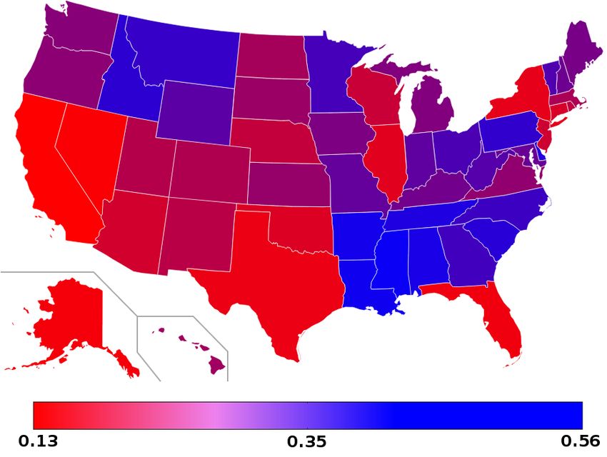
in the Twitter historical archives (and public API) average sentiment for each author, we need ourtextual variables to set the prior).
As it is not feasible to show the prior average
sentiment of all 57, 710 users, we created 20 even
sentiment bins, from −1.0 to 1.0. We then plot-
ted the number of users whose average sentiment
falls into these bins (Figure 8). Similar to other
variables, the positive end of the graph is much
heavier than the negative end.
Figure 5: Average sentiment of different hours of
the day in the USA, averaged across three years,
from 2012 to 2014.
Figure 7: Number of users (logarithmic) in bins of
50 tweets. The first bin corresponds to number of
users that have less than 50 tweets throughout the
three years and so on.
Figure 6: Average sentiment of different months in
the USA, averaged across three years, from 2012
to 2014.
sample size to not be too small. However, a large
number of the users in our dataset only tweeted
once or twice during the three years. Figure 7
shows the number of users in bins of 50 tweets. Figure 8: Number of users (with at least 50 tweets)
(So the first bin corresponds to the number of users per sentiment bins of 0.05, averaged across three
that have less than 50 tweets throughout the three years, from 2012 to 2014.
year.) The number of users in the first few bins
were so large that the graph needed to be logarith-
8 Results
mic in order to be legible. We decided to calcu-
late the prior sentiment for users with at least 50 We used 5-fold cross validation to train and eval-
tweets. This corresponded to less than 1% of the uate our baseline and contextual models, ensur-
users (57, 710 out of 7, 657, 158 total users). Note ing that the tweets in the training folds were not
that these users are the most prolific authors in our used in the calculation of any of the priors or in
dataset, as they account for 39% of all tweets in the training of the bigram models. Table 3 shows
our dataset. The users with less than 50 posts had the accuracy of our models. The contextual model
their prior set to 0.0, not favouring positive or neg- outperformed the baseline model using any of the
ative sentiment (this way it does not have an im- contextual variables by themselves, with state be-
pact on the Bayesian model, allowing other con- ing the best performing and day of week the worst.The model that utilized all the contextual variables are tagged with timestamps and author informa-
saw a 10% relative and 8% absolute improvement tion, so all the other four contextual variables used
over the baseline bigram model. in our model can be used for classifying the senti-
ment of any tweet.
Model Accuracy Note that the prior probabilities that we cal-
Baseline-Majority 0.620 culated need to be recalculated and updated ev-
Baseline-Bigram 0.785 ery once in a while to account for changes in the
Contextual-DoW 0.798 world. For example, a state might become more
Contextual-Month 0.801 affluent, causing its citizens to become on average
Contextual-Hour 0.821 happier. This change could potentially have an ef-
Contextual-Author 0.829 fect on the average sentiment expressed by the cit-
Contextual-State 0.849 izens of that state on Twitter, which would make
Contextual-All 0.862 our priors obsolete.
Table 3: Classifier accuracy, sorted from worst to 10 Conclusions and Future Work
best.
Sentiment classification of tweets is an important
Because of the great increase in the volume area of research. Through classification and anal-
of data, distant supervised sentiment classifiers ysis of sentiments on Twitter, one can get an un-
for Twitter tend to generally outperform more derstanding of people’s attitudes about particular
standard classifiers using human-labelled datasets. topics.
Therefore, it makes sense to compare the perfor- In this work, we utilized the power of distant
mance of our classifier to other distant supervised supervision to collect millions of noisy labelled
classifiers. Though not directly comparable, our tweets from all over the USA, across three years.
contextual classifier outperforms the distant super- We used this dataset to create prior probabilities
vised Twitter sentiment classifier by Go et al (Go for the average sentiment of tweets in different
et al., 2009) by more than 3% (absolute). spatial, temporal and authorial contexts. We then
Table 4 shows the precision, recall and F1 score used a Bayesian approach to combine these pri-
of the positive and negative class for the full con- ors with standard bigram language models. The
textual classifier (Contextual-All). resulting combined model was able to achieve
an accuracy of 0.862, outperforming the previ-
Class Precision Recall F1 Score ous state-of-the-art distant supervised Twitter sen-
Positive 0.864 0.969 0.912 timent classifier by more than 3%.
Negative 0.905 0.795 0.841
In the future, we would like to explore addi-
Table 4: Precision, recall and F1 score of the full tional contextual features that could be predictive
contextual classifier (Contexual-All). of sentiment on Twitter. Specifically, we would
like to incorporate the topic type of tweets into
our model. The topic type characterizes the na-
9 Discussions ture of the topics discussed in tweets (e.g., break-
ing news, sports, etc). There has already been ex-
Even though our contextual classifier was able tensive work done on topic categorization schemes
to outperform the previous state-of-the-art, dis- for Twitter (Dann, 2010; Sriram et al., 2010; Zhao
tant supervised sentiment classifier, it should be and Jiang, 2011) which we can utilize for this task.
noted that our contextual classifier’s performance
is boosted significantly by spatial information ex- 11 Acknowledgements
tracted through geo-tags. However, only about one
to two percent of tweets in the wild are geo-tagged. We would like to thank all the annotators for their
Therefore, we trained and evaluated our contextual efforts. We would also like to thank Brandon Roy
model using all the variables except for state. The for sharing his insights on Bayesian modelling.
accuracy of this model was 0.843, which is still This work was supported by a generous grant from
significantly better than the performance of the Twitter.
purely linguistic classifier. Fortunately, all tweetsReferences 1, pages 151–160. Association for Computational
Linguistics.
[Barbosa and Feng2010] Luciano Barbosa and Junlan
Feng. 2010. Robust sentiment detection on twit-
[Katz1987] Slava Katz. 1987. Estimation of prob-
ter from biased and noisy data. In Proc. COLING
abilities from sparse data for the language model
2010, pages 36–44. Association for Computational
component of a speech recognizer. Acoustics,
Linguistics.
Speech and Signal Processing, IEEE Transactions
[Bird et al.2009] Steven Bird, Ewan Klein, and Edward on, 35(3):400–401.
Loper. 2009. Natural language processing with
Python. O’Reilly Media, Inc. [Kouloumpis et al.2011] Efthymios Kouloumpis,
Theresa Wilson, and Johanna Moore. 2011. Twitter
[Bollen et al.2011] Johan Bollen, Huina Mao, and Al- sentiment analysis: The good the bad and the omg!
berto Pepe. 2011. Modeling public mood and emo- Proc. ICWSM 2011.
tion: Twitter sentiment and socio-economic phe-
nomena. In Proc. ICWSM 2011. [Mitchell et al.2013] Lewis Mitchell, Morgan R Frank,
Kameron Decker Harris, Peter Sheridan Dodds, and
[Chen and Goodman1999] Stanley F Chen and Joshua Christopher M Danforth. 2013. The geography of
Goodman. 1999. An empirical study of smooth- happiness: Connecting twitter sentiment and expres-
ing techniques for language modeling. Computer sion, demographics, and objective characteristics of
Speech & Language, 13(4):359–393. place. PloS one, 8(5):e64417.
[Chesley et al.2006] Paula Chesley, Bruce Vincent,
Li Xu, and Rohini K Srihari. 2006. Using verbs and [Moore2009] Robert J Moore. 2009. Twit-
adjectives to automatically classify blog sentiment. ter data analysis: An investor’s perspective.
Training, 580(263):233. http://techcrunch.com/2009/10/05/twitter-data-
analysis-an-investors-perspective-2/. Accessed:
[Csikszentmihalyi and Hunter2003] Mihaly Csikszent- 2015-01-30.
mihalyi and Jeremy Hunter. 2003. Happiness in ev-
eryday life: The uses of experience sampling. Jour- [Nakagawa et al.2010] Tetsuji Nakagawa, Kentaro Inui,
nal of Happiness Studies, 4(2):185–199. and Sadao Kurohashi. 2010. Dependency tree-
based sentiment classification using crfs with hidden
[Cui et al.2006] Hang Cui, Vibhu Mittal, and Mayur variables. In Proc. NAACL-HLT 2010, pages 786–
Datar. 2006. Comparative experiments on senti- 794. Association for Computational Linguistics.
ment classification for online product reviews. In
AAAI, volume 6, pages 1265–1270. [Oswald and Wu2011] Andrew J Oswald and Stephen
Wu. 2011. Well-being across america. Review of
[Dann2010] Stephen Dann. 2010. Twitter content clas- Economics and Statistics, 93(4):1118–1134.
sification. First Monday, 15(12).
[Davidov et al.2010] Dmitry Davidov, Oren Tsur, and [Pang et al.2002] Bo Pang, Lillian Lee, and Shivaku-
Ari Rappoport. 2010. Enhanced sentiment learning mar Vaithyanathan. 2002. Thumbs up?: sentiment
using twitter hashtags and smileys. In Proc. COL- classification using machine learning techniques. In
ING 2010, pages 241–249. Association for Compu- Proc. EMNLP 2002-Volume 10, pages 79–86. Asso-
tational Linguistics. ciation for Computational Linguistics.
[Diakopoulos and Shamma2010] Nicholas A Di- [Porter1980] Martin F Porter. 1980. An algorithm for
akopoulos and David A Shamma. 2010. Char- suffix stripping. Program: electronic library and in-
acterizing debate performance via aggregated formation systems, 14(3):130–137.
twitter sentiment. In Proc. SIGCHI 2010, pages
1195–1198. ACM. [Read2005] Jonathon Read. 2005. Using emoticons to
reduce dependency in machine learning techniques
[Fleiss1971] Joseph L Fleiss. 1971. Measuring nomi- for sentiment classification. In Proceedings of the
nal scale agreement among many raters. Psycholog- ACL Student Research Workshop, pages 43–48. As-
ical bulletin, 76(5):378. sociation for Computational Linguistics.
[Gallup-Healthways2014] Gallup-Healthways. 2014.
[Roy et al.2014] Brandon C Roy, Soroush Vosoughi,
State of american well-being. Well-Being Index.
and Deb Roy. 2014. Grounding language models
[Go et al.2009] Alec Go, Lei Huang, and Richa in spatiotemporal context. In Fifteenth Annual Con-
Bhayani. 2009. Twitter sentiment analysis. En- ference of the International Speech Communication
tropy, 17. Association.
[Jiang et al.2011] Long Jiang, Mo Yu, Ming Zhou, Xi- [Saif et al.2012] Hassan Saif, Yulan He, and Harith
aohua Liu, and Tiejun Zhao. 2011. Target- Alani. 2012. Alleviating data sparsity for twitter
dependent twitter sentiment classification. In Proc. sentiment analysis. CEUR Workshop Proceedings
ACL 2011: Human Language Technologies-Volume (CEUR-WS. org).[Sriram et al.2010] Bharath Sriram, Dave Fuhry, Engin
Demir, Hakan Ferhatosmanoglu, and Murat Demir-
bas. 2010. Short text classification in twitter to im-
prove information filtering. In Proc. ACM SIGIR
2010, pages 841–842. ACM.
[Vosoughi2014] Soroush Vosoughi. 2014. Improv-
ing automatic speech recognition through head pose
driven visual grounding. In Proceedings of the
SIGCHI Conference on Human Factors in Comput-
ing Systems, pages 3235–3238. ACM.
[Wang et al.2011] Xiaolong Wang, Furu Wei, Xiaohua
Liu, Ming Zhou, and Ming Zhang. 2011. Topic
sentiment analysis in twitter: a graph-based hashtag
sentiment classification approach. In Proc. CIKM
2011, pages 1031–1040. ACM.
[Zhao and Jiang2011] Xin Zhao and Jing Jiang. 2011.
An empirical comparison of topics in twitter and tra-
ditional media. Singapore Management University
School of Information Systems Technical paper se-
ries. Retrieved November, 10:2011.You can also read