Estimating Arbitrage Profits for Storage Resources in Nodal Electricity Markets: A Decision Tree Method

Estimating Arbitrage Profits for Storage Resources in Nodal Electricity
Markets: A Decision Tree Method

 Devendra Canchi, Monitoring Analytics LLC., +1 765 603 6498, devcanchi@gmail.com
 Benjamin Fram, Norwegian School of Economics (NHH), +47 4123 1477, benjamin.fram@nhh.no

Overview
As the share of power generation from intermittent wind and solar plants is projected to grow in the coming decades,
there is increasing recognition among industry participants that a variety of low-carbon power storage resources will
also grow to manage this intermittency. There remain, however, ongoing discussions about the profitability of these
storage resources and at what point market conditions will support widespread investment in utility-scale storage
applications. In most restructured wholesale power markets, the profitability of a storage resource will depend on its
ability to arbitrage intraday price differences by purchasing power at low prices and selling it at higher prices.

In this paper, we propose an optimal strategy for a utility scale storage operator to maximize arbitrage profits in a nodal
market with intraday price variation. We use this approach to compute the expected profit and profit distribution for a
representative set of generation pricing nodes in the wholesale electric power market operated by the Midcontinent
Independent System Operator (MISO). We draw several useful insights by weighing the geographical distribution of
arbitrage profit potential against the underlying variables contributing to the price volatility in the Midcontinent ISO.
Finally, we examine the sensitivity of the arbitrage profit potential to the two defining operational specifications of the
storage facility: capacity and round trip efficiency.

Arbitrage Potential

In the United States, nearly 60 percent of electric power is bought and sold in markets managed by Independent System
Operators (ISO) using marginal pricing principles. The ISOs continuously match load by dispatching generation
resources in the merit order subject to transmission and reliability constraints. The prices, known as locational marginal
prices (LMPs) or nodal prices, are set by the ISO at select locations or nodes using marginal pricing principles. The
pricing mechanism ensures that the nodal prices generally track the offer curve with high prices during periods of high
demand such as early mornings and late evenings and low prices during periods of low and intermediate demand,
which span most of the night time, late mornings, and afternoons. The markets have also evolved over time. In addition
to reflecting the marginal cost of incremental demand, most nodal prices in wholesale power markets today also include
various penalties imposed by the ISOs to incentivize a reliable operation of the grid. In some locations, the penalties
largely contribute to price spikes that range from 10 to 40 times the average nodal price. The increased penetration of
intermittent resources has also contributed to the intraday price variation and expensive backup generation needed to
balance the load during a rapid decrease in wind or solar generation also contributes to higher prices. Lastly, a variety
of market pricing rules such as those designed to manage the congestion with neighboring markets or balancing
authorities also contribute to the frequency and magnitude of the intra-day price variation. These varying intraday
prices create arbitrage opportunities for storage operators. A storage operator would profit by buying power from the
grid when the prices are low and selling power back to the grid when the prices are high. Without perfect foresight,
however, a storage operator’s challenge is to devise an optimal strategy to arbitrage uncertain intraday prices.

Literature Review
Using storage resources to arbitrage intraday prices in wholesale electricity markets has been suggested since the
beginning of the restructuring era that paved the way to the adoption of locational marginal pricing. Walawalkar et al.
[2007] proposed a simple strategy (charging during off peak hours and discharging during peak hours) to profit from

energy price arbitrage and frequency regulation in the New York area. Similar approaches were used by Sioshansi et
al. [2009], Zafirakis et al. [2016] and Byrne and Silva [2012]. Paatero and Lund [2005], Kim and Powell [2011] and
Barnhart et al. [2013] all examined pairing intermittent resources with storage resources. Krishnamurthy et al. [2017],
Jiang and Powell [2016] introduced optimal bidding strategies in the day-ahead market to maximize a storage
resource’s arbitrage profits.

Mathematical Formulation
We propose an optimal arbitrage strategy for a storage resource offering directly in the real time market with ex-ante
pricing. Our approach assumes that the storage resource would offer in the real time market directly. In most nodal
markets, the intraday price variation in the real time markets (and therefore profit potential) is substantially higher than
the intraday price variation in the day-ahead market. In addition, in most restructured nodal electric power markets,
the real time market prices are ex-ante, meaning that the prices paid to the generators are known at the beginning of
the settlement interval. This allows the storage operator to react to prices in real time. A storage operator with a fast
response time could begin to discharge if the real time price spikes.

We assume that at the beginning of every settlement interval, the storage operator’s choices are: charge, discharge, or
remain idle for the interval. In markets with ex-ante settlement prices, the nodal price for the settlement interval is
revealed to the storage operator. We assume that the revealed price also signals the future price trajectory for the
remaining decision time horizon. We further assume that the prices are Markov: future prices are conditioned only on
the revealed price of the most recent settlement interval.

Figure 1 Example of a Price Trajectory

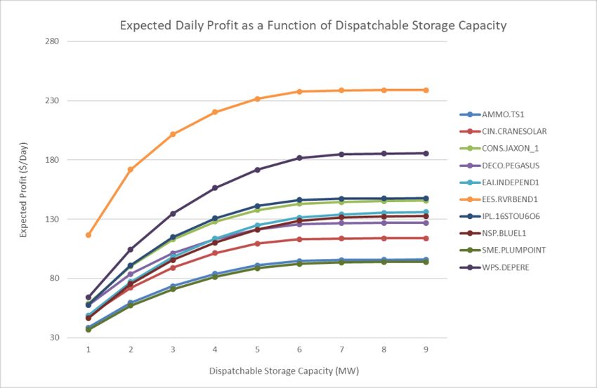
Figure 1 shows an example price distribution faced by the storage operator. The price at the beginning of the settlement
interval 1 ($ 0 per MWh) is known to the storage operator. Hence 0 is trivially equal to 1. The distribution of price
for the next settlement interval 2 ($ 1 per MWh with 1 probability and $ 2 per MWh with 2 probability, 1 + 2 =
1) is conditioned on the price of the settlement interval 1 . The distribution of price for the settlement interval 3 is
conditioned on the price of the settlement interval 2 . For every settlement interval, the unconditional probabilities
follows as: 1 = 0 ∗ 1 , 2 = 0 ∗ 2 , 3 = 0 ∗ 1 ∗ 2 , 4 = 0 ∗ 1 ∗ 4 , 5 = 0 ∗ 1 ∗ 5 and 6 = 0 ∗ 2 ∗
 6 .

The goal of the storage operator is to maximize the arbitrage profit given the conditional price distribution subject to
capacity constraint and round trip efficiency of the storage resource.

Let for ∈ represent the decision space for the storage operator. In the simple illustrative example shown in Figure
1, = {0,1,2,3,4,5,6}. For convenience, we define a mapping function ℘( ) to represent the prior decision point for a
given decision point . In the simple illustrative example shown in Figure 1, ℘(1) = 0, ℘(5) = 2.

For each , is the price to buy or sell electric power and is the unconditional probability of realizing . We
define, , ∈ {0,1}, as a binary variable to represent the decision to charge and , ∈ {0,1}, as another binary
variable to represent the decision to discharge. To simplify, we further define , = − , ∈ {−1,0,1}, as an
integer variable representing the decision to discharge ( = 1), charge ( = −1) and stay idle ( = 0 ). Lastly, we
define , ≥ 1, to represent the total charge available in the reservoir. Hence, the total charge is net of all charge and
discharge decisions made at prior decision points leading to the decision point . In the simple illustrative example
shown in Figure 1, 3 = 0 + 1 + 3 .

For a storage resource with loss factor , minimum operating capacity , maximum operating capacity , and
initial level of charge in the reservoir , we formulate the operators problem of maximizing the expected arbitrage
profit in a market with ex-ante pricing as follows.1

 ∑ ∗ ∗ ( − ∗ ) (1)
 
Subject to

 0 = (2)

 ∀ , = ℘( ) + (3)

 ∀ , ≤ ≤ (4)

The equation 2 ensures the available charge in the reservoir for the first decision point is equal to the initial level of
the charge in the reservoir. The equation 3 ensures that the total charge in the reservoir at every decision point is equal

1
 Loss Factor is defined as 1+ (1-Efficiency Factor). For example, the loss factor for a storage resource with a
round trip efficiency of 80 percent is 1.2.

to the net of all prior charge and discharge decisions. The equation 4 ensures that the total charge in the reservoir at
every decision point does not fall outside of the specified capacity bounds of the storage resource.

The expected arbitrage profit from the solving the storage operator’s charge-discharge-stay-idle mixed-integer problem
follows.

 ( ∗ ) = ∑ ∗ ∗ ( ∗ − ∗ ∗ ) (5)
 
The distribution of arbitrage profits could also be derived from solving the storage operator’s charge-discharge-stay-
idle problem. Let for ∈ ; ⊂ represent the terminal decision points in the decision space for the storage operator.
In the simple illustrative example shown in Figure 1, = {3,4,5,6}. Let ∗ represent the optimal arbitrage profit for
the storage operator following the decision path that terminates at . In the simple illustrative example shown in Figure
1, the decision path through 0, 1 and 4 terminates at 4. The arbitrage profit ∗ is the sum total of profits earned at every
decision point in the path leading to the terminal decision point .

 ∗ ∗ ∗ ∗
 ∗ = ∗ ( ∗ − ∗ ∗ ) + ℘( ) ⋅ ( ℘( ) − ∗ ℘( ) ) + ℘(℘( )) ∗ ( ℘(℘( )) − ∗ ℘(℘( )) )+ (6)
 ….

The probability of realizing ∗ is same as the probability of following the decision path that terminates at the decision
point .

 ( ∗ = ∗ ) = ∗ ℘( ) ∗ ℘(℘( )) ∗ …. (7)

Computational Complexity

The storage operator’s charge-discharge-stay-idle problem presents a formidable computational challenge. The number
of decision points increase exponentially with the number of price states. For instance, there are 2.2x10 21 decision
points in a 24 hour problem involving seven discrete price states. We propose an alternative approach. We break down
the storage operator’s problem into multiple sub-problems using Bellman equations and solve recursively to obtain the
optimal sequence of charge, discharge and stay-idle decisions (see Bellman [1957]). A formal proof is provided in the
appendix A.

Empirical Analysis
The Midcontinent Independent System Operator

To empirically test our model, we chose to use real world market data from the Midcontinent Independent System
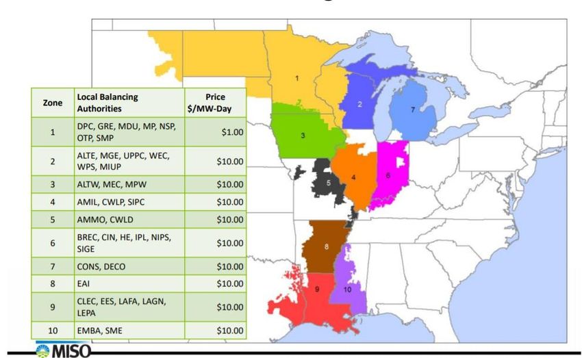
Operator (MISO), which serves large swaths of the American Midwest and Central South regions. Figure 2, which was
taken directly from an official MISO market report, depicts the MISO market footprint.

Figure 2. The MISO Market Footprint

 https://cdn.misoenergy.org/2018-19%20PRA%20Results173180.pdf

The MISO is subdivided into ten Load Resource Zones (LRZs) that roughly correspond to state borders, but deviate
from these borders to more closely match service territories of transmission owners (TOs), also called Local
Balancing Authorities (LBAs). Figure 2 also lists the LBAs whose service territories are contained within each LRZ.

Data Acquisition

From the MISO website, we downloaded hourly real time prices for all 1,586 generation pricing nodes in the MISO
during the time period beginning January 1st, 2017 and ending December 31st, 2020. This yielded approximately 48.0
million observations of hourly real time price observations.

In order to account for cyclical daily and seasonal load patterns, we then sorted prices for each node into two different
categories: weekdays and weekends/NERC holidays. NERC holidays are major federal holidays in the US where the
demand for power is typically lower than a normal working day during the week. We then further subdivided both the
weekday and weekend categories into four groups; Quarter 1 (Q1), which spans January through March; Quarter 2
(Q2), which spans April through June; Quarter 3 (Q3), which spans July through September; Quarter 4 (Q4), which
spans October through December. As a result of this sorting, we end up with eight groups of hourly real time prices:
Q1 weekdays, Q1 weekends, Q2 weekdays, Q2 weekends, and so on.

Calculating Seven Price States

To perform our empirical analysis, we create seven distinct price states from the raw hourly real time prices. To capture
the leptokurtic nature of real time power prices, we choose five states to comprise the middle 96 percent of the price
distribution and two additional states that replicate the lower and upper bounds or “spikes” of the price distribution.
To do this, we first calculated price quantiles at each individual node quantile increments of 0.05. We then calculated
the 0.0, 0.005, 0.01, 0.15, and 0.02 quantile values of the price distribution at each node and calculate the mean of this
interval to capture the “fat tail” price at the low end of the distribution. We take the mean of the 0.98, 0.985, 0.99,
0.995, and 1.0 quantiles to calculate the high price spikes at the high end of the distribution. We calculated the mean
values between 0.02 and 0.2, 0.2 and 0.4, 0.4 and 0.6, 0.6 and 0.8, and 0.08 and 0.98 to create the price levels in
between the high and low values. Then, depending upon in which quantile interval it falls, we assign each observed
hourly price at each node one of the seven calculated price state values.

As a simple example, assume the price at a node was $20/MWh at 12:00 on a given day, the price was $22/MWh at
13:00, and the price was $100/MWh at 14:00. Assume prices at 12:00 and 13:00 both fall within the 0.2-to-0.4 quantile

price interval and the price at 14:00 falls into the 0.98-to-1.0 interval. Then both the prices at 12:00 and 13:00 are
assigned the same price value ($22.13/MWh as an example) and the price at 14:00 will take on the value of the top 2
percentile ($87.45/MWh as an example). Thus, each of the observed prices is assigned one of seven calculated values
that correspond to the approximate quantile of the original price. For each pricing node, we create seven price states
for each of the eight time periods. For instance, we create seven price states for all nodes for Q1 weekdays, seven price
states for Q3 weekends, and so on. This gives us a total of fifty-six price states for each node.

Filtering Out Time-Deficient and Duplicate Nodes

To ensure that we can compare the results from our analysis, we first filter out nodes with an insufficient number of
observations. We choose to filter out nodes that have less than 50 percent of the possible hourly observations or are
missing observations in one of the eight seasonal/weekday subgroups. This brings the number of nodes for our
empirical analysis down to 1,350.

It is common practice for ISOs to assign multiple pricing nodes to the same generating facility. For example, if a gas
fired combustion turbine consists of three separate combustion turbine units, the ISO may assign three pricing nodes
to the same generator, one for each unit. The ISO does this in case one unit is unoperational but in reality, the nodal
prices co-located at one generator will be identical. In addition, sometimes multiple entities own partial shares of the
same generating unit and the ISO will again assign duplicate nodes to the same generator. To reduce the time spent
computing profitability across nodes and time periods, we grouped together all nodes with less than a $0.01/MWh
difference across all fifty-six price states and chose one representative node per group. This filtration reduces the 1,350
price nodes left from the first round of filtering down to a total of 856 “unique” nodes. We are therefore left with
approximately 29.8 million hourly price observations for our empirical analysis.

Optimization Model Runs

For all 856 unique MISO price nodes, we compute the optimal profit and profit distribution using the optimization
mode developed earlier. All ISOs use five minute settlements to manage real time markets. The hourly price is not
fully revealed to the storage operator until the beginning of the last five minute settlement period. We assume that the
hourly transition matrix is an unbiased approximation to the more granular five minute transition matrix. There are 23
transitions within an operating day. We assume that are transition probabilities are not independent of the time of the
hour in the day. The transition probability from second price state to the third price state in the hour ending four is not
necessarily same as the transition probability from second price state to the third price state in the hour ending six.

For each of the 856 unique MISO price nodes, we estimated transition probability matrices for the eight representative
days in a year. In other words, we separately estimated the transition probability matrix for each quarterly weekday
and weekend separately. For each representative day, we estimated the unconditional probabilities for the first hour
and conditional (transition) probabilities for the remaining subsequent 23 hours. We assume that the inter-day transition
probabilities, i.e., from the last hour of the prior day to the first hour of the next day, is negligible.

Given the estimated probability matrix and prices, we optimized the storage operators, charge, discharge or stay-idle
decision for each representative day using the optimization formulation described above. The mixed integer
optimization is divided into multiple sub-problems and solved recursively using Bellman equations. We obtained the
expected profit and probability distribution of the profit for every selected pricing node for each representative day.

Monte Carlo Simulations - Yearly Profit Distribution

We also derived the yearly profit distributions for the storage operator for all selected pricing nodes from their
respective eight representative day profit distributions using Monte Carlo simulation. For every day, a random profit
is drawn from the corresponding representative day’s profit distribution. The total profit for the year is obtained by

adding the daily profits. We simulated 5,000 iterations to derive the yearly profit distribution for every selected pricing
node.

Results
Profitability and Statistical Properties of Nodal Prices

After collecting the results of our empirical analysis, we first investigate if there exist any patterns between node
profitability and a series of statistical measurements of the nodal prices. For each of the eight representative days used
in our analysis, we calculated the mean, median, standard deviation, skewness, kurtosis, and range of prices at all 856
nodes used in the analysis. We then graph the relationships between expected storage resource profitability and the
statistical measurements of prices at the corresponding node.

These graphs reveal several patterns. First, there are strong, positive--sloping linear patterns between the standard
deviation of prices at a node and the expected profitability. This relationship holds across all eight representative days.
We fit simple OLS trend lines to measure the relationship between these two variables and see R-squared values
ranging from 0.770 for Q1 weekends to 0.941 for Q3 weekends. Figure 3 below

 Figure 3. Daily Profit as a Function of Nodal Price Standard Deviation for a 3MW Battery - Q3 Weekdays

In addition, there are also strong, positive-sloping linear correlations between the price range at a given node and the
expected profitability. Again, this relationship holds across all eight representative days although the strength of the
relationship varies more than that between profitability and standard deviation. The highest R-squared value between
range and profitability 0.914 for Q2 weekdays and the lowest is 0.736 for Q3 weekdays.

Finally, we see no discernable patterns between expected profitability and mean, median, skewness, or kurtosis values
of prices at a given node. We believe that it makes intuitive sense that statistical measurements of spread are positively
correlated with higher profits for storage resources that seek to make money via price arbitrage. Larger and more
frequent differences in prices provide more opportunities for storage resources to buy and sell at high profits.

Geographic Distribution of Profitable Nodes

In the MISO, we see clear geographic patterns in node profitability. Figure 4 below ranks all 856 nodes used in the
Monte Carlo simulation from highest (1) to lowest (856) profitability and maps them to the LRZ in which they lie.

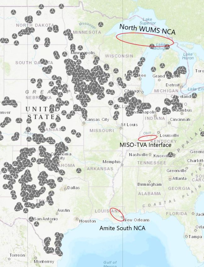
Figure 4. Location of Profitability-Ranked Nodes in MISO

Immediately, we see that the hundred most profitable nodes are clustered in LRZ 9, LRZ 2, and LRZ 6. Upon further
inspection of these results, we see that the highly profitable nodes in LRZ 9 correspond to a group of power plants that
lie on the Mississippi river between Baton Rouge and New Orleans in southwestern Louisiana. Many of these plants
are coal and gas-fired units located near heavy industrial sites that sit along this stretch of river. As it turns out, this
area is designated as the Amite South Narrowly Constrained Area (NCA) by the MISO. NCA’s are special designations
for areas of the grid with frequently binding network constraints and especially volatile prices. The cluster of highly
profitable nodes in LRZ 2 correspond to the Northern Wisconsin-Upper Michigan (NWUMS) NCA where sparse
transmission lines can cause similar problems. The cluster of plants in LRZ 6 are coal plants located in the Big River
Electricity Company territory in Western Kentucky that abets a market interface with the Tennessee Valley Authority
(TVA). We suspect that volatility at these pricing nodes might be caused by Transmission Line Loading Relief (TLR)
maneuvers that have been reported to cause congestion in the interface between MISO and TVA (Potomac Economics
(2020)).

In addition, we see that LRZ 7 and remaining nodes in LRZ 9 are clustered heavily towards the more profitable end of
the spectrum. We suspect nodes in LRZ 7 might exhibit higher profitability due to the Lake Erie Loop Flow between
MISO, PJM Interconnection, the New York ISO, and Ontario ISO (IESO) that regularly impacts Michigan. We suspect
that market interface issues between the Texan wholesale market (ERCOT) and the Eastern part of Texas/Louisiana
that lie in MISO might be driving profitability in the LRZ 9.

Profitability by Fuel Type

From the results both our optimization model Figure 5. Map of Wind Resources in MISO and
calculations of expected profits and Monte Carlo Most Profitable Node Clusters (Circled in red)
simulations of annual profits, we see no clear
relationship between the type of generator technology
located at a given pricing node and the expected
profitability of the node. Steam coal power plants are
scattered widely throughout the MISO footprint although
they are less frequent in LRZ 10, which is conterminous
with western and southern Mississippi. The same is true
for gas-fired power plants with the exception of Northern
Minnesota, Northwestern Wisconsin, and North Dakota.

Figure 5 shows the distribution of wind generators in the
MISO market footprint. In contrast to coal, gas, and
nuclear generators, wind generators in the MISO are
heavily clustered in the states of Iowa (LRZ3), southern
Minnesota (LRZ1) and central Illinois (LRZ4). Figure 5
also includes the three market regions that, combined,
contain 71 of the top 100 most profitable nodes from our
Monte Carlo analysis: the Amite South NCA, North
WUMS NCA, and Southern Indiana/Western Kentucky
border between MISO and TVA. Taking into account the
strong correlation between arbitrage profitability and
price volatility from our results, the lack of any clear
pattern between node profitability and fuel type of the
generator located at the corresponding pricing node Source: EIA U.S. Energy Mapping System
strongly suggests that extreme price volatility in the https://www.eia.gov/state/maps.php
MISO is driven more so by binding transmission network
constraints and market interface modelling issues. Given
the tendency for storage advocates to cite pairing storage
resources with intermittent renewables, we believe that this is an important result that merits further discussion as this
pairing may not necessarily offer storage resource investors the highest return for their investment. In the MISO, it
appears that installing a battery at most wind turbines will lead to sub-optimal returns in comparison to alternative
nodes.

Storage Capacity

We ran a series of sensitivity analyses on our model to test the impact of changing storage capacity on expected
profitability. Figure 6 depicts the expected daily profitability of a storage resource located at ten representative nodes
located throughout the MISO footprint. Figure 6 shows expected profits as a function of dispatchable storage capacity.
For instance, since our model assumes that the storage resource must maintain a minimum of 1 MW of charge, a value
of “1” on the x-axis on this graph indicates that the resource has a total installed capacity of 2 MW. All optimization
runs to create these profitabilities assumed a 20 percent round-trip efficiency and the ability to charge or dispatch 1
MW every hour.

Figure 6. Expected Daily Profit as a Function of Dispatchable Storage Capacity

We see very clearly in Figure 6 that profitability increases as storage capacity but at a decreasing rate. For most nodes,
profitability appears to largely flatten our when the dispatchable capacity reaches 6 MW and stop increasing entirely
at 7 MW.

We believe that this result can be explained by looking more closely at the number of average arbitrage opportunities
a storage resource can expect to have on a daily basis. Figure 7 shows the hourly coefficient of variation (COV), i.e.
the standard deviation divided by the mean, for prices at all nodes in the MISO from the entire sample period of 2017-
2020. Because the storage resource is assumed to have a roundtrip efficiency of 80 percent, the red horizontal line
depicts the minimum COV that a storage resource would need to sell power at a profit if they purchased power at a 0.6
COV. Similarly, the blue horizontal line depicts the level at which they would need to sell power at a profit if they
purchased power at a price of 0.7.

 Figure 7. Coefficient of Variation for All Hourly Real Time Nodal Prices in MISO

We see that there are six price COVs that lie about the blue line and four that lie between the red and blue lines. To
make a significant profit, the storage resource would want to sell power above the blue line. Since there are six COVs
that lie above this line, it would make sense that, on average, the storage resource can earn a significant profit during
six hours of the day. They could make a profit by selling at a point that lies above the red line as well but it would
mean they had to purchase power at a COV level of 0.6. It therefore makes sense that marginal profitability will
approach zero as the storage resource’s capacity approaches 7 MW.

Conclusion

In this paper, we present an intertemporal profit maximization problem for a storage resource participating in a
restructured wholesale electricity market with nodal pricing. This storage resource seeks to maximize profits via
arbitrage in the real time energy market, i.e. by charging when power prices are low and selling power back into the
grid when prices are high. Prices are assumed to follow a discrete Markov process with seven possible states. To
capture underlying market dynamics, the price states change from low to high between hours according to a series of
twenty-four transition probability matrices. The storage resource also faces operational constraints such as storage
capacity limits, round-trip charge/discharge efficiency, and minimum charge levels. These operational constraints
impact its decision to charge, discharge, or remain idle when faced with current and expected future price states.

To empirically test our model, we use hourly real time market prices from the Midcontinent ISO (MISO) to estimate
the expected profitability and accompanying profitability distributions for a storage resource. These raw data are used
to create the price levels and transition probability matrices for the profit maximization problem. We sort these data
into seasons and peak/off-peak days and then calculate expected profitability across 856 unique price nodes in MISO
. We also run Monte Carlo simulations to calculate the annual expected profitability at these nodes.

The results of our empirical analysis reveal several trends. First, we see that the expected profitability of a storage
resource at a given node is highly correlated with the standard deviation and range of the prices at that node. In the
MISO, we see that the nodes with the highest expected profitability are clustered in geographic regions where
insufficient transmission network infrastructure leads to frequent congestion issues and volatile prices. The Amite
South Narrowly Constrained Area (NCA) located in Southwestern Louisiana and the Northern WUMS NCA in the
Michigan Upper Peninsula accounted for forty-five and nineteen of the top one hundred most profitable nodes
respectively in the Monte Carlo simulation. In addition, seven of the top one hundred most profitable nodes were
located in southern Indiana and western Kentucky. These nodes are located close to the market interface between
MISO and TVA, an area that has had documented interface modeling issues leading to price spikes in MISO. We see
no patterns between the fuel type of a generator at a given pricing node and profitability for the storage resource. In
fact, the majority of pricing nodes at wind turbines are located in LRZ1 and LRZ3, both of which contain nodes heavily
clustered in the bottom half of the profitability distribution. LRZ1 in particular contains sixty-nine of the one hundred
least profitable nodes in our analysis. This pattern stands in stark contrast to the notion that storage resources can
achieve their highest profits when coupled with intermittent renewables. Our empirical results instead suggest that the
most profitable use of storage resources might be to balance market areas that frequently experience network
congestion and exhibit high price volatility.

We believe there are a number of exciting avenues for future research that could further shed light on the profitability
of storage resources. One avenue would be to use a portfolio optimization approach to maximize the profits of a fleet
of batteries operating in a single market. This would build directly off the evidence presented in this paper that the
expected profitability of a storage resource is highly correlated with the volatility of the prices where it is located. A
portfolio of storage resources could allow investors to maximize their expected return while also taking into account
their appetite for risk. In this paper, we assumed that a storage resource operator would be focused primarily on real
time nodal prices since they typically exhibit considerably higher price spreads than day ahead market prices. Though
we are comfortable with our decision to focus on real time prices, it could be worthwhile to investigate how storage

resources could improve profitability by participating in the day ahead energy market as well. Finally, storage
resources, and batteries in particular, are slowly becoming more prevalent in ancillary service markets. In the United
States, batteries already participate in regulation submarkets due to their ability to respond quickly to fluctuations in
system frequency and help system operators manage power imbalances on the power grid. Important research remains
to be done to determine how storage resources should operate to maximize profits in these ancillary service markets.

Appendix A
Consider a simple binomial decision tree that represents the options available for a storage operator. At each decision
node, the storage operator has to decide whether to charge or discharge or idle.

Figure 2 Decision Tree

 , ∈ {0,1,2,3,4,5,6} represents the decision nodes

The mapping function ℘( ) provides the prior decision node to the decision node . For example, ℘(1) = 0, ℘(5) =
2.

 , ∈ {0,1}, a binary variable represents the decision to charge

 , ∈ {0,1}, a binary variable represents the decision to discharge

 , = − , ∈ {−1,0,1}, a integer variable represents the decision to discharge ( = 1), charge ( = −1)
and stay idle ( = 0 )

 , > 0 represents the loss factor

 , 0 ≤ ≤ 1 represents the probability of the decision node . For each time period, the probabilities sum to 1.
For example, 1 + 2 = 1; 3 + 4 + 5 + 6 = 1.

 , represents the expected price at the decision node 

 ∗ represents the expected price at the decision node 

 , ≥ 1, represents the total charge available in the reservoir at a decision node . The total charge at a decision
node is net of charge and discharge decisions at all nodes leading to the decision node . For example, 3 = 0 +
 1 + 3 .

 represents minimum capacity and represents maximum capacity of the reservoir.

The storage operator’s goal is optimally charge and discharge so as to maximize the expected profits.

 ( ∗ , 0 , , ), represents the maximum profit that storage operator could earn given the expected
prices, starting level of the reservoir and capacity limits of the reservoir.

The optimal profit for the full tree, ( ∗ , 0 , , ) is obtained by solving the following mixed integer
problem

 ( ∗ , 0 , , ) =

 ∑ ∗ ∗ ( − ∗ ) (A1)
 
Subject to

 0 = 1 (A2)

 = ℘( ) + (A3)

 ≤ ≤ (A4)

Alternatively, ( ∗ , 0 , , ) is obtained by solving a two-step mixed integer problem.

In the first step, the conditional optimal profits for sub branch 5 and 6 are obtained. In the second step, the optimal
profit for residual tree is obtained by using the sub branch conditional optimal profits obtained in the first step.

The sub branch optimal profit for a given , ∈ { 1 , 2 , 3 , … }, is obtained by solving the following
mixed integer problem

 ( 5 ∗ 5 , 6 ∗ 6 , , , ) =

 5 ∗ 5 ∗ 5 + 6 ∗ 6 ∗ 6 (A5)

Subject to

 + 5 = 5 (A6)

 + 6 = 6 (A7)

 ∀ ∈ {5, 6} ≤ ≤ (A8)

The optimal profit for the residual tree, ( ∗ , 0 , , ) is obtained by solving the following mixed
integer problem.

 ( ∗ , 0 , , ) =

 ∑ ∗ ∗ + ∑ ∗ ( 5 ∗ 5 , 6 ∗ 6 , , , ) (A9)
 ∉{5,6} 
Subject to

 0 = 1 (A10)

 ∀ ∉ {5,6}, = ℘( ) + (A11)

 ∀ ∉ {5,6}, ≤ ≤ (A12)

 ∑ ∗ = 2 (A13)
 
 ∑ = 1 (A14)
 
 ∈ {0,1} (A15)

Proposition: ( ∗ , 0 , , ) ≡ ( ∗ , 0 , , )

Proof

Part 1: Objective functions for both formulations are equivalent

From (9)

 ∑ ∗ ∗ + ∑ ∗ ( 5 ∗ 5 , 6 ∗ 6 , , , ) (A16)
 ∉{5,6} 

Following (5),

 ∑ ∗ ∗ + ∑ ∗ [ 5 ∗ 5 ∗ 5 + 6 ∗ 6 ∗ 6 ] (A17)
 ∉{5,6} 

Following (14)

 (A18)

 Following (14)

 ∑ ∗ ∗ + [ 5 ∗ 5 ∗ 5 + 6 ∗ 6 ∗ 6 ]
 ∉{5,6}

The above objective function (A18) is identical to the objective function (A1) specified in the full tree formulation.

Part 2: Feasible sets for both formulations are equivalent

Setting any arbitrarily selected, equal to 1, constraints (A13) through (A15) can be expressed as

 2 + 5 = 5 (A19)

 2 + 6 = 6 (A20)

Proof:

Given (A14) and (A15),

 1 = 0; 2 = 0; … . = 1; … −1 = 0; = 0 (A21)

Substituting in (A13),

 1 ∗ 1 + 0 ∗ 2 + ⋯ 1 ∗ + ⋯ 0 ∗ −1 + 0 ∗ = 2 (A22)

Simplifying further,

 = 2 (A23)

Substituting for in constraints (6) and (7) of the sub problem

 2 + 5 = 5 (A24)

 2 + 6 = 6 (A25)

The two constraints (A24) and (A25), combined with the remaining constraints, constraint (A8) of the sub branch
problem formulation and constraints (A10) through (A12) of the residual problem formulation are identical to
constraints (A2) through (A4) of the full tree problem formulation.

Since the objective function and constraints are identical, the formulations are equivalent.

References
C. J. Barnhart, M. Dale, A. R. Brandt, and S. M. Benson. The energetic implications of curtailing versus storing
solar- and wind-generated electricity. Energy & Environmental Science, 6(10): 2804–2810, 2013.

R. E. Bellman. Dynamic Programming. Princeton University Press, Princeton, NJ, USA, 1957.

R. H. Byrne and C. A. Silva-Monroy. Estimating the maximum potential revenue for grid connected electricity
storage: Arbitrage and regulation. Tech. Rep. SAND2012-3863, Sandia National Laboratories, 2012.

Jiang, D.R., W.B. Powell. 2015. Optimal hour-ahead bidding in the real-time electricity market with battery storage
using approximate dynamic programming. INFORMS Journal on Computing 27(3) 525–543.

J. H. Kim and W. B. Powell. Optimal energy commitments with storage and intermittent supply. Operations
Research, 59(6):1347–1360, 2011.

D. Krishnamurthy, C. Uckun, Z. Zhou, P. Thimmapuram, and A. Botterud, “Energy storage arbitrage under day-
ahead and real-time price uncertainty,” IEEE Transactions on Power Systems, 2017.

J. V. Paatero and P. D. Lund. Effect of energy storage on variations in wind power. Wind Energy, 8(4):421–441,
2005.

Potomac Economics. “2019 State of the Market Report for the MISO Electricity Markets.” June 2020.
https://www.potomaceconomics.com/wp-content/uploads/2020/06/2019-MISO-SOM_Report_Final_6-16-20r1.pdf

R. Sioshansi, P. Denholm, T. Jenkin, and J. Weiss, “Estimating the value of electricity storage in pjm: Arbitrage and
some welfare effects,” Energy economics, vol. 31, no. 2, pp. 269–277, 2009

R. Walawalkar, J. Apt, and R. Mancini. Economics of electric energy storage for energy arbitrage and regulation in
New York. Energy Policy, 35(4):2558–2568, 2007.

D. Zafirakis, K. J. Chalvatzis, G. Baiocchi, and G. Daskalakis, “The value of arbitrage for energy storage: Evidence
from european electricity markets,” Applied Energy, vol. 184, pp. 971–986, 2016.