Fast constraint satisfaction problem and learning-based algorithm for solving Minesweeper
←
→
Page content transcription
If your browser does not render page correctly, please read the page content below
Fast constraint satisfaction problem and
arXiv:2105.04120v1 [cs.AI] 10 May 2021

                                                   learning-based algorithm for solving
                                                               Minesweeper
                                          Yash Pratyush Sinha1 , Pranshu Malviya1, and Rupaj Kumar Nayak1
                                           1
                                               International Institute of Information Technology Bhubaneswar, India

                                                                                  Abstract

                                                     Minesweeper is a popular spatial-based decision-making game that works
                                                 with incomplete information. As an exemplary NP-complete problem, it is
                                                 a major area of research employing various artificial intelligence paradigms.
                                                 The present work models this game as Constraint Satisfaction Problem (CSP)
                                                 and Markov Decision Process (MDP). We propose a new method named
                                                 as dependents from the independent set using deterministic solution search
                                                 (DSScsp) for the faster enumeration of all solutions of a CSP based Minesweeper
                                                 game and improve the results by introducing heuristics. Using MDP, we im-
                                                 plement machine learning methods on these heuristics. We train the classi-
                                                 fication model on sparse data with results from CSP formulation. We also
                                                 propose a new rewarding method for applying a modified deep Q-learning
                                                 for better accuracy and versatile learning in the Minesweeper game. The
                                                 overall results have been analyzed for different kinds of Minesweeper games
                                                 and their accuracies have been recorded. Results from these experiments
                                                 show that the proposed method of MDP based classification model and deep
                                                 Q-learning overall is the best methods in terms of accuracy for games with
                                                 given mine densities.

                                         1 Introduction
                                         Minesweeper is a single-player game where the player has been given a grid mine-
                                         field of size p × q containing n mines where each block of the grid contains at
                                         most one mine. These mines are distributed randomly across the entire minefield
                                         and their locations are not known to the player. The goal of the game is to uncover
                                         all blocks which do not contain a mine (i.e., all safe blocks). If a block containing

                                                                                      1
a mine is uncovered, the player loses the game. Whenever a safe block is uncov-
ered, it represents the number of mines in its 8-neighbors containing mines. In the
human version of the game, when this number is zero the game automatically un-
covers all of the 8-neighbours of such a block. Generally, the first block uncovered
by the player does not contain a mine. Analyzing the given pattern and arrange-
ment of these boundary digits, the player has to figure out the position of the safest
block that can be uncovered. The player can also mark a block with a flag if he/she
decides that the block is mined. In this way, the number of mines left to be dis-
covered is updated and the player can continue to play until all the free blocks are
revealed. In some situation, if there exists one than one block with similar chances
of containing a mine, but not with the surety of absence of mine, the player has
to randomly choose the next block to uncover. As a result of this ambiguity, the
player can lose the game even if he applies the most optimal strategy. As it is com-
putationally difficult to make an optimal decision without considering all options,
Minesweeper is an NP-complete problem [13] which is an intriguing area of re-
search. Many researchers have already described the formulation techniques that
can be employed for this game and improved upon the previous ones as discussed
in the next section.

2    Related Work
A strategy called the single-point strategy considers only one instance of the un-
covered block and finds the safest move from its immediate neighbours. Its imple-
mentation model may vary but the single point computations are common practice
in them. As a result, this strategy struggle with larger dimensional games or games
with higher mine densities. Therefore, other strategies can be used to reconcile
the limitations of single-point techniques. CSP is another prominent way of for-
mulating the Minesweeper game in a mathematical form and several algorithms
[22] exist to solve these CSPs. CSPs are the subject of intense research in both AI
and operations research since not only it overcomes the problems in single-point
strategy, but the regularity in their formulation provides a common basis to analyze
and solve problems of many unrelated families [11, 4]. MDP is another way of
formulating games into state-action-reward form. This way has been extensively
practised nowadays to formulate games [15]. We also use such a formulation and
combines it with the CSP formulation to achieve even better results.
     Realizing the Minesweeper game as a CSP as described in [20] is one of the
basic ways that is employed as discussed. The thesis by David Becerra [2] tests
and talks about several different approaches are taken to solve the Minesweeper
game and comes to the conclusion that CSP methods work as efficiently as any

                                          2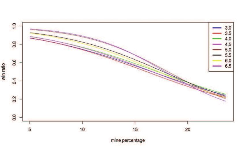
other formulations of the Minesweeper game.
     Our method for solving CSPs is in line with the look-ahead method proposed
by Dechter and Frost [10] that avoids unnecessary traversal of the search space to
result in a more optimized method for dealing with CSPs.
     The work of Bayer et al. [1] describes another approach that uses generalized
arc consistency and higher consistencies (1-RC & 2-RC) to solve the CSP gener-
ated by the Minesweeper to assist a person playing a game of Minesweeper. Both
of these approaches are inefficient when constraints are not very scalable for larger
boards.
     Nakov and Wei [17] describes the Minesweeper game as a sequential decision-
making problem called Partially Observable Markov Decision Problem (POMDP)
and convert the game to an MDP, while also reducing the state space.
     Approaches have been carried out like using belief networks by Bonet and
Geffner [3] that consider a set of partially observable variables and considers the
possible states as beliefs.
     In the research by Castillo and Wrobel [6] authors described methods to learn
the playing strategy for Minesweeper not just by inferring from a given state but
also by making an informed guess that minimizes the risk of losing. They used
Induction of Logic Program (ILP) techniques such as macros, greedy search with
macros, and active inductive learning for the same. This is very different from
another machine learning approach that we have used which is also very promising.
     Sebag and Teytaud [19] have attempted to estimate the belief states in the
Minesweeper POMDP by simplifying the problem to a myopic optimization prob-
lem using Upper Confidence Bounds for Monte-Carlo Trees (UCB for Trees).
While this method is reasonably accurate for small boards, it is too slow for larger
board sizes making it inadequate. As described in research of Legendre et al. [14],
authors have used heuristics with computing probabilities from CSP called HCSP
to study the impact of the first move and to solve the problem of selecting the
next block to uncover for complex Minesweeper grids based on various strategies.
By preferring the blocks which are closest to the frontier in case of a tie on the
probability of mines, they got the better results for various sizes of Minesweeper
matrices. We have also used a variant of HCSP by using Manhattan distance for
measuring closeness to the boundary.
     In the research given by Buffet et al. [5], authors combined the two methods
i.e., UCB for trees and HCSP as described in [19] and [14] respectively to improve
the performance of UCB to be used not only for small boards but also for big
Minesweeper boards. This improves performance by a lot.
     Recent works by Couetoux et al. [9] have tried to solve Minesweeper by di-
rectly treating it as a Partially Observable MDP (POMDP).
     However, as pointed out by Legendre et al., Minesweeper is actually a Mixed

                                         3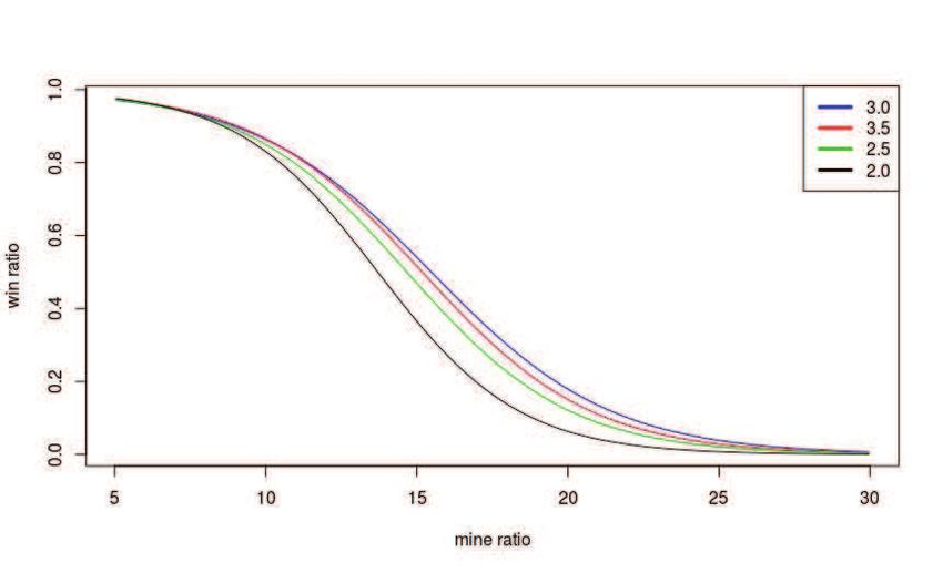
Observability MDP (MOMDP) and several improvements can be made to the cur-
rent solvers to increase performance.
     In the research of Gardea et al. [12] the authors have taken an approach to
utilize different machine learning and artificial intelligence techniques like linear
and logistic regression and reinforcement learning.
     Q-learning [21] is a reinforcement-learning algorithm which has been used ex-
tensively in games [15, 16] to solve MDPs. We have also used a modified version
of the Q-learning for solving the above MOMDP efficiently.
     In this paper, we have described our methods of creating an automatic solver
for Minesweeper using several techniques by gradually improving upon its pre-
vious ones. We have also used a modified version of Q-learning for solving the
above MOMDP efficiently. In section 2, we describe how the game is formulated
into CSP and then in an MDP. We describe techniques to play the game using both
the CSP & MDP formulation. Also, we have described three ways to obtain the
probabilities of each block containing a mine as well as a method to find blocks
about which we can deterministically say if they contain a mine. After that, we give
several methods, both hand-crafted and machine learning-based to choose blocks
in the case that there is no deterministic solution. In section 4 we described the
implementation of these methods and present the results graphically and a com-
parison table with existing popular methods. We conclude the paper in section
5.

3    Formulations
Prior to the detailed explanation of algorithms and machine learning techniques
that we used, in this section, we are going to describe how the minesweeper game
is first realized as a playable mathematical form. These forms and notations then
allowed us to design and improve upon the existing algorithms, particularly for
this game for better results. This paper particularly uses two different formats,
expressing the game as a CSP or as an MDP.

3.1 CSP formulation
CSP [22] is a natural and easy way for the formulation of minesweeper, as it accu-
rately captures the intuition of finding which blocks may or may not contain a mine.
We use the fact that each uncovered block shows the number in its 8-neighbour re-
gion in order to build a CSP from the minesweeper game. These numbers put
a constraint on the covered blocks in the neighbourhood that how many of them
should have a mine. (We also know the total number of mine present in the game.

                                         4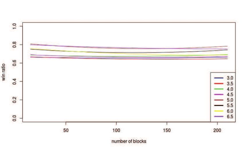
This information will be used as heuristics discussed later in the paper.) If we treat
the covered blocks as boolean variables (with 0 representing a safe block and a
1 representing a mine) we can use the uncovered numbers as constraints on such
variables. For example, a two uncovered block will constrain the sum of all of
the variables in its eight neighbours to two. Assuming the uncovered number of
every block at (i, j) represented by numi,j and the boolean variables represented
by minei,j , the constraints can be written as (adaptively for blocks on the border):
                                j+1
                            i+1 X
                            X
                numi,j =                 minek,l if (k 6= i & l 6= j)               (1)
                           k=i−1 l=j−1

    For several (i, j) we will obtain a set of the equation in the form of equation
(1). We can re-write this set of equations in a matrix format as follows:

                                      AM = N,                                       (2)

Where M is the vector denoting a list of uncovered variables, N is the list of all
applicable numi,j and A is a binary coefficient matrix obtained from equation (1).

3.2 MDP formulation
Markov Decision Process (MDP) is formulating the minesweeper game as 5−tuple
of (S, A, T, R· (·, ·), γ) where

    • S is a set of all the possible states of the game that represents all the possible
      board configurations at any time. It includes a special state sinit which is
      the initial state of the game as well as the final states slose and swin which
      represents the state when the game is lost and the state of winning the game
      respectively.

    • A is the set of all actions that can be performed at any time on a state s to
      go to some next state s′ . For minesweeper, this represents all the covered
      blocks that can be uncovered to go from the current board state to the board
      state after the block has been uncovered.

    • T is the set of transition triplets (s, a, s′ ) which is the probability of going
      to the next state s′ from the current state s by doing the action a. In our
      consideration, the probability for a being 1 means the player is surely going
      to lose.

    • R is the reward function R(s, a) representing the reward to be received after
      performing action a on a state s. Our model rewards an action a according

                                           5
to the number of blocks that are deterministically uncovered after it is per-
formed, as we want to encourage the model to choose the action which would
uncover the maximum number of blocks with the least chance of losing the
game.
• γ is the discount factor according to which the future rewards are reduced.
A POMDP is a more general way of formulating the game as it captures the
intuition that the entire state is not observable. POMDPs are solved by using belief
states, which are generally computed using simulations or other tree search meth-
ods with bs,a = b(s, a, s′ ) where bs,a is the belief on state s on taking action a
and observing state s′ . This entire method, however, overlooks the fact that a part
of the state is fully observable making the problem a Mixed Observability MDPs
(MOMDPs). MOMDPs are generally easier and faster to simplify and solve than
POMDPs. Our method uses this fact while ignoring the non-observable part of this
MOMDP in the belief state to further simplify this problem. Since we neglect both
the hidden part of the state and the future observation in this belief, we call it a
sub-state denoted by sa = b(s, a). Here b is a function that takes a section of the
board as a subset, based on the action. This sub-state is dependent on the current
state and the action to be performed only. The details of how and what sub-states
have been used are given in section 3.2.
4 Solving Method
This section contains strategies to find the next best block to uncover. Our solu-
tion is based on a two-step process. The first step is called Deterministic Solution
Search (DSS), which evaluates solutions for the backbone variables (whose value
is the same in all solutions) if they exist for equation (2). DSS collects all deter-
ministic variables which satisfy the constraints in the equation (2) and assigns them
to be uncovered. The other non-deterministic variables are ignored.
In this way, we do not have to go for any other methods to find the safest
block each time. This method proves to be very effective as it has a worst-case
time complexity to O(n2 m). The steps to find deterministic variables are given in
Algorithm 2.
Now, if Algorithm 2 returns a non-empty vector there exists some determined
blocks which can directly uncover them or flag.
But if it is found that there is no such deterministic variable, we move to the
next step. The primary approach of a player is to select the next move based on
current knowledge of the state and thus we estimate the probabilities of each block
being safe or unsafe.
6Algorithm 1 : Reduce(A,N,j,value)
1: if value is 0 then
2: Set column j of A to 0
3: else if value is 1 then
4: Reduce value of Nj by 1
5: Set column j of A to 0
6: end if
Algorithm 2 : DSS(A,M,N)
1: Detrmined ← empty list
2: loops ← Any significanly large number, say 10
3: for loops number of times do
4: for Each row i in A do
5: V ariables ← Number of variables in Ai
6: if V ariables is 0 then
7: Delete row Ai from A
8: else if Ni is 0 then
9: for every variable vari,j = 1 in Ai do
10: Reduce(A, N, j, 0)
11: Add variable Mj with value 0 to to Determined
12: end for
13: else if V ariables = Ni then
14: for every variable vari,j = 1 in Ai do
15: Reduce(A, N, j, 1)
16: Add variable Mj with value 1 to to Determined
17: end for
18: end if
19: end for
20: end for
21: Return Determined
74.1 From CSP
We propose approaches to find a set of feasible solutions for the CSP formulated
using equation (2) using which the probabilities for non-deterministic variables are
estimated. We generate a solution set by either using a simple backtracking method
or by our proposed DSScsp algorithm where both algorithms require traversing of
a tree.
• The first one is to use backtracking that constructs a pruned tree where the
path for every deepest leaf node is one possible solution. The tree is tra-
versed recursively to gather solutions that satisfy the given set of constraints
or equation (2). This was implemented mainly to compare with our proposed
method.
Algorithm 3 : DSSCSP(A,M,N)
1: Static S ← empty list
2: if A is a Zero-Matrix then
3: M is a possible solution, add it to S
4: end if
PM
5: i = argmaxi∈M ( j i j); where Mi is ith column in M
6: A′ , M ′ , N ′ = A, M, N
7: Mi′ = 0
8: if A′ M ′ = N ′ is possible then
9: Reduce(A′ , N ′ , i, Mi′ )
10: Run DSS(A′ , M ′ , N ′ ) for further reduction
11: DSSCSP (A′ , M ′ , N ′ )
12: end if
13: A′′ , M ′′ , N ′′ = A, M, N .
14: Mi′′ = 1
15:
16: if A′′ M ′′ = N ′′ is possible then
17: Reduce(A′′ , N ′′ , i, Mi′′ )
18: Run DSS(A′′ , M ′′ , N ′′ ) for further reduction
19: DSSCSP (A′′′ , M ′′ , N ′′ )
20: end if
21: Return S
• DSScsp, as given in Algorithm 3, uses DSS, in the Algorithm 2, at each
step, to quickly reduce the backtracking search space. The depth of the tree
is drastically reduced as several variables are resolved in a single node due
8to DSS. This leads DSScsp being randomized and much faster than simple
backtracking in general. The Reduce function in Algorithm 1 is used in both
Algorithm 2 and Algorithm 3.
Using one of these ways, we now have a set of solutions, or a solution matrix
S that satisfy the given constraint equation (2). To limit the time taken to find these
equations, we have employed a strategy of just computing a random large enough
subset of all the possible solutions over the full set of solutions. We do this by
setting a maximum number of solutions, a maximum depth as well as a maximum
number of iterations. The guarantee of the sample being random comes from the
fact that, in DSScsp we assign values 1 or 0 randomly.
This set of solutions allows us to compute the probabilities of a block contain-
ing a mine.
Ps Ps Ps
⊤ i=1 S1,i i=1 S2,i i=1 Sm,i
P = , , ... , (3)
s s s
where, S represents the binary solution matrix and s is the number solutions
generated. In S matrix, each row corresponds to a unique solution to equation (2)
i.e., Si,j = 1 only if block j contained a mine in solution i.
The simplest way to proceed with the game after obtaining probabilities is to
uncover the block with the least probability of having a mine. But there are ways to
improve. We developed several heuristics in addition to these probabilities that play
a crucial role and employed machine learning algorithms to have faster execution
with more accuracy.
However, in Minesweeper, even the supposedly best move picked by any heuris-
tic, might result in losing the game.
4.2 Heuristic approaches
We have built heuristics that consider the problem using several other parameters
and formulations like the size of the board, total number of mines, flags used,
the location of blocks etc. which may affect the results. We have used machine
learning to find the best heuristics with these parameters.
4.2.1 Manhattan Distance
Legendre et al.[14] consider a heuristic that the blocks closer to the edges of the
board are likely to be more informative about blocks involved in equation (2) as
compared to the farther ones. We consider the same and use the manhattan distance
between block at (i, j) to the nearest edge of the board. We also relax the rule of
9choosing the block with minimum probability. Instead, we choose a list of blocks
Bs such that ∀m ∈ Bs : Ps ≤ min(P ) + 0.05 where min(P ) is the minimum
probability in P , and P is the vector of probabilities of a block containing a mine
(3). Now that we have a reduced list of safe blocks, we choose the one with the
minimum manhattan distance from the minefield boundary. We uncover this block
now.
4.2.2 Supervised Learning
This method follows a machine learning approach in which we define the given
situation as a state and uncovering a block as a action. It is a binary classification
model that is trained on the different states and their corresponding actions taken
in Minesweeper game. We collect the data from the games played randomly by
the previous versions. The aim is to classify the action as safe or unsafe for the
current state. We divide the collected data as xtrain and ytrain as follows.
• xtrain : The input part x that describes the information we know from the
current state and an action. It consists of the following:
– Size of the board (p, q)
– Number of mines
– Coordinates of the covered blocks (i, j): These are the coordinates of
the covered blocks in the neighbor (variable boundary) of uncovered
blocks. We also consider 3 random covered blocks in current state.
– Probability (p): The probability is the same as obtained from DSS-
csp algorithm if the covered block lies in the variable boundary in the
current state. Otherwise, its value is assigned to 0.5 as there is no
information given for that block.
– Size of M .
– Variable with minimum probability (index(pmin )): It is the index (action)
of the covered block from the variable boundary with minimum prob-
ability of having mine.
– Score(corner/edge/middle): It is the additional heuristic we use in this
method. We take the probability of a block to have no neighboring mine
into account so that more blocks can uncover and we get better and
more detailed view of the game from the new state. In other words,
we are considering the next immediate state of the minesweeper game
just after we click a block. This score varies as per the orientation of
the new block on the board:
10If f is the number of flags already used and l is the number of uncov-
ered blocks left,
m−f 4
Score(Mij = 0 | (i, j) = corner) = 1 − ( )
l
m−f 6
Score(Mij = 0 | (i, j) = edge) = 1 − ( ) (4)
l
m−f 8
Score(Mij = 0 | (i, j) = middle) = 1 − ( )
l
As corner block will have the maximum score, it will uncover the larger
area of the board that eventually increase chances of winning the game.
• ytrain : The output part consists of a single column corresponding to each
data point in xtrain as y. Its value is 1 if the block turns out to be safe or else
it is 0.
We then propose to train two machine learning models with the above data.
XGBoost: Single-pass Classification Here, we have implemented binary clas-
sification of above state-action pair represented as xtrain into classes of win and
loss as ytrain . We use single-pass eXtreme Gradient Boost (XGBoost) [7] classifier
to do this. It is an ensemble technique that is used to build a predictive tree-based
model for handling sparse data where the model is trained in an additive manner.
Here, new models are created that predict the residuals or errors of prior models and
then added together to make the final prediction. So, instead of training one strong
learning algorithm XGBoost trains several weak ones in a sequence until there is
no further improvement. The objective of XGBoost is based on loss function L(θ)
(we use logistic for binary classification) for prediction and a regularization part
R(θ) (we use L2 regularization) that depends on the number of leaves and their
prediction score in the model that control its complexity and avoids overfitting.
Let the prediction yipred for a data-point xi be,
yipred =
X
θj xij . (5)
j
Here θj are learned by the model from data. Considering mean squared error, loss
function for actual value yi will be,
(yi − yipred )2 .
X
L(θ) = (6)
i
Hence, the objective function for XGBoost mathematically is,
Obj(θ) = L(θ) + R(θ). (7)
11We optimize the above objective function by training from the given data and the
model tune its parameter accordingly. When the model is trained with the data, at
every new state we test the above data as input to and the model returns a predicted
score, y pred , such that 0 ≤ y pred ≤ 1, where, larger the value of y pred , more is the
chance of that block to be safe. Hence for each state, we select the block with the
maximum score, to uncover and proceed to another state.
Neural Network: Here, classification is done by iteratively generating a small
batch of data and training the model with it. This method allows the model to learn
and adapt according to the randomly generated data. The model is a simple multi-
layer neural network for binary classification that takes x as its input and returns y
as output. Table 1 describes the neural network layers, the number of neurons in
them and the corresponding activation functions.
We used the Relu activation function for all layers except the output layer that
uses the Sigmoid activation function as y is between 0 and 1. Here, the loss was
evaluated using binary cross-entropy for its logistic behaviour and optimizer as
Adam. These configurations were done after experimental validation. Our model
of iterative classification was inspired by the experience-replay training methods.
In this, however, we just train the model iteratively in a given number of episodes
by generating the training data using the previously made model. Algorithm 4
describes the iterative process of training the neural network.
Table 1: Neural Network
Layer Number of Neurons Activation Function
Input sizeof(x) ReLU
Hidden1 sizeof(x) ReLU
Hidden2 5 ReLU
Hidden3 5 ReLU
Output 1 sigmoid
4.2.3 Q-Learning
We use the MDP formulation as described in section 2.2 as a heuristic. As stated
there, we have avoided state space explosion by using sub-states instead of belief
states. The advantage of using a sub-state over a belief state is that a sub-state can
be calculated only using the current state and the expected action. Belief states,
on the other hand, need to be calculated by trying to predict the observation, often
requiring expensive tree search methods to be computed. It should be pointed out
that while our actual formulation is a MOMDP, we have ignored the unknown
12Algorithm 4 : Iterative Classification
1: Import weights from current model
2: nepisodes ← number of episodes
3: batch ← 10
4: for each episode from 1 to nepisodes do
5: xtrain , ytrain ← make data(batch)
6: Train model with xtrain and ytrain
7: Save updated model and weights
8: end for
belief part to improve on computability. In our formulation, these sub-states are
of a fixed size sub × sub with the centre of the sub-state representing the block
to be uncovered (i.e., the action). We then use deep Q-learning to solve the MDP
formulated earlier by learning a Q-function to predict expected discounted reward
and we then choose the action with the maximum expected discounted reward.
In Q-learning, we train a model to learn a Q-function given its inputs. The form
of Q-function used in our application is given in the equation (8). The Q-function
will take the same amount of time for every board configuration irrespective of
the size of the board. This makes it such that the limitation here is the number of
possible actions which is the number of uncovered blocks. This Q-learning can
find the next action in O(pq) where p and q are the dimensions of the given board.
computation. The transition rule of Q-learning (SARSA) is given as:
Q(sa , a) = R(sa , a) + γ max
′
Q(s′a′ , a′ ) (8)
a
Here, sa represents the sub-state of state s for choosing any action a, s′ and a′
represents the state at after choosing action a.
However, the problem exists that the direct sub-state is not very representative
of the expected reward for any action. For this, we use a score as defined in equa-
tion (9) to represent every covered block in the sub-state. The score is designed
such that it retains information of its safe probability as well as its location. For a
number to represent location we have used the formula in equation (4).
Sci,j = α × Pi,j + (1 − α) × scorei,j (9)
Here Pi,j represent the probability of mine being present at (i, j), scorei,j represent
the location score and α is a variable to be chosen such that the Sci,j represents the
best possible score. We have used any invalid values to represent an uncovered
block. In order to decrease bias in α, we have defined it as a linear function of
13n
board dimension (p & q) and mine ratio p×q .
n
α = θ1 × p + θ2 × q + θ3 × + θ4 . (10)
p×q
To obtain an α which would give us a good representation of the score, we
obtained win ratios of different values of α by playing with the heuristic given in
section 4.2.1 on the vector of Sc instead of P . We then performed linear regression
with the α which maximized win ratio as the target to obtain the values of θ1 to
θ4 . By using the method described above, we can obtain scores Sci,j for every
block (i, j). Using these scores, we can find a sub-state of size sub × sub for each
action a where each element of the sub-state is the score in Sc. We then defined
the immediate reward R(sa , a) for any action a as in equation (11).
number of newly opened blocks because of action a
R(sa , a) = . (11)
(p × q) − n
We then ran several simulations to find the net discounted expected reward
Q(sa , a) for several action a sub-state sa pairs. A neural network of the configura-
tion given in Table 2 was then trained to predict the Q-function. As done in section
4.2.2, both single-pass training and iterative training methods were used. We then
choose the action which maximizes the expected discounted reward Q(sa , a).
Table 2: Network for Q-function
Layer Number of Neurons Activation Function
Input sub × sub ReLU
Hidden1 sub × sub tanh
Hidden2 sub × sub linear
Hidden3 sub × sub linear
Output 1 tanh
5 Experiment
For the experiment, we implemented the minesweeper game from scratch along
with a playable interface in C++. We then built the various versions of the solver in
which every version (except version 6.5 and 3.0) is an improvement over the previ-
ous version with a new algorithm or tuned parameters. The versions are numbered
as given in Table 3.
By creating several different versions of the solver we were able to see the
performance improvement caused by each subsequent algorithm.
14Table 3: Versions with algorithm description
Version Number Algorithm
1.0 Backtracking
2.0 1.0+DSS
2.5 1.0 limited + DSS
3.0 DSScsp + DSS
3.5 DSScsp limited + DSS
4.0 3.0 + Manhattan Distance
4.5 3.5 + Manhattan Distance
5.0 4.5 + Supervised Learning using Single-pass Classification
5.5 4.5 + Supervised Learning using Iterative Approach
6.0 4.5 + Q-Learning using Iterative Classification
6.5 4.5 + Q-Learning using Single-pass Classification
5.1 Formulating as CSP
All versions from 2.0 to 4.5 were implemented in C++ for faster performance.
Backtracking with DSScsp was implemented iteratively to avoid stack overflow as
version 2.0. Version 2.5 is the limited traversal of the search tree by limiting the
depth and width to be traversed in the search tree. The width is limited by limiting
the number of solutions to 100. The depth is limited by limiting the number of
swaps, or the number of edges starting from the root node of the tree to 1000. We
choose the number of solutions as 100 as it gives reasonably accurate results, in
much less time.
Version 3.0 is the implementation of DSScsp Algorithm 3 along with Algo-
rithm 2 to find the solution set. This method finds the same solution set as simple
backtracking. Hence, it has the same accuracy as that in Version 2.0. But, it is
much faster in terms of time taken to solve the Minesweeper game.
Version 3.5 is the limited traversal of the search tree traversed in Version 3.0.
The time taken is reduced by limiting the depth and breadth of the search tree. The
limitations are chosen such that accuracy and amount of time are similar in the case
of version 3.5 and version 2.5. We have set the limit to the number of solutions to
100 and limit to the depth of the tree to 300, such that the accuracy of Version 3.5
remains almost similar to version 3.0 while reducing the total amount of time.
Versions 4.0 and 4.5 are the extensions of versions 3.0 and 3.5 respectively.
They include the heuristic rules defined in section 4.2.1.
155.2 Formulating as MDP
We used the machine learning method to perform classification that utilizes the in-
formation like state − action pair and their corresponding result. We denote this
information as one data-point. The data was collected by playing games using ver-
sion 4.0, with x-dimension of board i.e., p, varying from 5 to 30 and y-dimension
i.e., q, as 0.5 × p to p. For each board, we generated at most 100 different mine
distribution possible in it. The mine ratios for these boards is varied from 5% to
30%.
5.2.1 Classification
For version 5.0, we collected this ample amount of data of around 23.3 million
and trained it using XGBoost classifier. We used the xgboost library in Python to
implement this model and save the trained model as a binary file. This binary file
is then accessed in C++ to play the game with version 5.0.
For version 5.5, we collected a batch of data of more than 0.7 million samples
similar to the previous version and trained the binary neural network (Table 1).
We saved the updated neural network model and then again generated a new batch
of data to repeat this process for 100 episodes. With each iteration, the weights
got updated and the model learned to classify dynamically. We built the neural
network model using keras [8]. As keras is a Python library, we used another
library keras2cpp [18], which allowed us to use the trained keras model in C++ as
a function.
5.2.2 Deep Q-Learning
In the versions 6.0 and 6.5, the first step to build the sub-state was to get parameters
as in equation (10) for a good value of α. This was done by first simulating several
games on different values of α as described in section 4.2.3. We varied α from 0
to 1 with increments of 1/30 for board configuration with the larger dimension 5
to 10 and 20 with mine ratio from 0.5 to 0.25 playing 100 games in each. We then
ran linear regression as in equation (10) with α which gave the maximum win ratio
with respect to the board size configuration and mine ratio. The regression gave an
r-squared value of 0.27 and thus was accurate.
On obtaining α we get the score for each block using equation (9) which we
could then used to build sub-states of sub = 3. For running the simulation to
obtain discounted rewards several games were played where the net reward and the
action-sub-state pair was recorded. Each reward was calculated as given in section
4.2.3.
16For the discount, we have used a linearly increasing discount over an exponen-
tially increasing discount so as to punish actions which may lead to a loss severely.
This converges as all our rewards are between 0 − 1, but the discounting factor can
increase to any number.
To obtain the simulations, as in section 4.2.2, we have used manhattan distance
as a base heuristic. We simulated various games with 5 to 20 and 30 with mine
ratios from 0.05 to 0.30 and playing 200 different games on each configuration.
For each game, we recorded the sequence of a sub-state-reward pair, where the
reward was the full discounted reward calculated after the game was over and the
sub-state is a vector of length 9 denoting the sub-state.
Since the sub-state captures information from both the state and action, a neural
network of the configuration in the table (2) built using keras and was trained to
learn the sub-state vector-reward mapping with mean squared error as the loss and
rmsprop as the weight optimizer. Using this as the first training pass, we then
used the model obtained above to get more reward-sub-state pairs from the model
obtained after training as described above and trained the model in an iterative
model. The iterative training was done on 50 episodes of the larger dimension of
5 to 20 and 30 with mine ratios from 0.05 to 0.20 and playing 5 games on each
configuration. This gave us the iterative pass trained model.
5.3 Results
In this section, we study the performance of each version by simulating them on
several minesweeper boards. In this way, we can have exact performance statistics
for each version for their interpretation and comparison. We compare the win
ratios of these methods and their dependencies on the mine ratio, the number of
blocks and the dimensional ratio of the board. The performance data is collected
by simulation of games where board size is changing from 5 to 15 with dimensional
ratio 0.5 (rectangular-board) to 1 (square-board). For all these configurations of the
boards, the mine ratio is set to vary from 5% to 25% with time out of 5 seconds
for each game. As the winning accuracy almost converges to 0 after decreasing
the density of mines reaches around 25% in any minesweeper board, we can get an
illustrative view of this logistics behaviour.
As of version 1.0, it is simple backtracking, it takes a lot of time to execute and
thatś why we do not consider it for comparison with other algorithms. In fig. 1, we
compare the winning accuracy of version 2.0 with versions up to 3.5 with respect
to different mine ratios. We can interpret from the figure that, version 2.0 performs
the worst, as it takes more than 5 seconds (computationally very slow) to solve that
causes frequent times out. The accuracy of versions 2.5 and 3.5 are very close to
that of 2.0 and 3.0 due to limited traversal. Overall, version 3.0 performs much
17better than others such as version 2.0, version 2.5 and version 3.5.
This difference in time taken is also illustrated in fig. 5 which shows how much
slower is version 2.0 as compared to version 3.0. Notice that with very high mine
percentages, version 2.0 begins to lose fast (as the games become harder) making it
less accurate. The same figure also shows that the limited versions such as version
2.5 and version 3.5 are much faster than the others, with a very low difference in
accuracy as seen from fig. 1. Noted that the negative values of time are a result of
cubic regression. We compared the performance of version 3.0 with other versions
to analyze the effects of adding heuristics in fig. 2 for same Minesweeper boards.
The heuristic in section 4.2.1 is experimentally proved to be useful for better results
as we notice an improvement in version 4.0 over 3.0 which is also evident from fig.
1.
If we talk about MDP formulations, one of the heuristics we use is the number
of mines left for a state in a game that results in further improvement in the accu-
racy. Now, as the number of total mines, n, is increased for a board, that is, the
mine ratio increase, the effect of left mines on the result decreases. Hence, versions
from 5.0 to 6.5 also produce similar results as previous versions and this was also
seen in fig. 2 with mine ratio above 19%. Overall, due to over-fitting, version 5.0
and 6.5 outperforms all other versions with a visible difference with 5.5 and 6.5
following them.
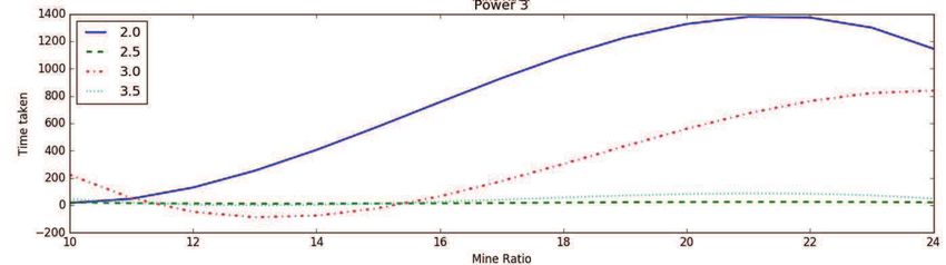
We also analyze the relationship between the win ratio of these algorithms with
a number of blocks in the board, p × q in fig. 4 as well as dimensional ratio, pq in
fig. 3 and find that it does not affect the overall accuracy of any versions as such.
The mine configuration of size 9 × 9 with 10 mines is considered as a standard
beginner size board. The accuracy obtained by algorithms presented in this paper
compared to [5] is given in Table 4.
6 Conclusion
In this paper, we have used the realization of the Minesweeper game as an MDP
and as a CSP to create several kinds of solving methods. We introduced DSScsp
(Algorithm 3), which can enumerate all solutions of the CSP much faster than
backtracking while being just as accurate. We also introduce the concept of limited
traversal which obtains a subset of all possible solutions and showed that it gives
nearly as accurate results as full traversal, while being much faster. We improved
preexisting heuristics (Version 4.0) and introduced new ones which used machine
18Figure 1: Mine ratio vs. win ratio in CSP based algorithms
Figure 2: Mine ratio vs. win ratio for all versions in table (3)
19Figure 3: Win ration vs ratio of length to breadth (p : q) of the minesweeper board.
Lower ratios indicate more “rectangularly” as opposed to higher ratios representing
”squareness”
Figure 4: Win ratio vs Number of total blocks in minefield. (p × q)
20Figure 5: Time vs mine percentage; Part of the graph goes to negative time due to
cubic regression limits
Table 4: Standard Beginner Board Accuracy
Version Number Accuracy
2.0 82.14
2.5 77.34
3.0 82.20
3.5 82.20
4.0 86.24
4.5 86.22
5.0 92.02 (max)
5.5 89.21
6.0 87.58
6.5 91.41
OH [5] 89.9
learning and deep Q-learning (Version 5.0 & version 6.5) on the MDP formulation
of the game which we showed to be better than that of existing methods (Table (4)).
We also showed that deep Q-learning is marginally better than machine learning
(classification) methods in general, but not always as can be seen in the Table
(4). Overall, we claim that our method of deep Q-learning (Version 6.5) can play
Minesweeper to a high degree of accuracy while still being fast enough to play
boards as large as 200 total blocks.
21References
[1] K. Bayer, J. Snyder, and B. Y. Choueiry. An interactive constraint-based
approach to minesweeper. pages 16–20, July, 2006.
[2] D. Becerra. Algorithmic approaches to playing minesweeper. 2015.
[3] B. Bonet and H. Geffner. Belief tracking for planning with sensing: Width,
complexity and approximations. In Journal of Artificial Intelligence Re-
search., 50:923–970, 2014.
[4] N. Bouhmala. A variable depth search algorithm for binary constraint satis-
faction problems. 2015.
[5] O. Buffet, C. S. Lee, W. Lin, and O. Teytaud. Optimistic Heuristics for
MineSweeper. In International Computer Symposium, Hualien, Taiwan,
2012.
[6] L. P. Castillo and S. Wrobel. Learning minesweeper with multirelational
learning. In Proceedings of the 18th International Joint Conference on Arti-
cial Intelligence, pages 533–538, August 2003.
[7] Tianqi Chen and Carlos Guestrin. Xgboost: A scalable tree boosting system,
2016.
[8] François Chollet. keras. https://github.com/fchollet/keras, 2015.
[9] A. Couetoux, M. Milone, and O. Teytaud. Consistent belief state estimation,
with application to mines. In International Computer Symposium, 2012.
[10] R. Dechter and D. Frost. Backjump-based backtracking for constraint satis-
faction problems. In Artificial Intelligence. v.136, 2002.
[11] M. Fellows, T. Friedrich, and D. Hermelin. Constraint satisfaction prob-
lems: Convexity makes all different constraints tractable. In Proceedings of
the Twenty-Second International Joint Conference on Artificial Intelligence,
2011.
[12] L. Gardea, G. Koontz, and R. Silva. Training a minesweeper solver. An
Autumn CS, 229, 2015.
[13] R. Kaye. Minesweeper is np-complete. In The Mathematical Intelligencer,
22:9–15, 2000.
22[14] M. Legendre, K. Hollard, O. Buffet, and A. Dutech. Minesweeper: Where to
probe? RR-8041, INRIA, 2012.
[15] V. Mnih, K. Kavukcuoglu, D. Silver, A. Graves, I. Antonoglou, D. Wier-
stra, and M. Riedmiller. Playing atari with deep reinforcement learning.
https://arxiv.org/abs/1312.5602, 0:1, 2013.
[16] Volodymyr Mnih, Koray Kavukcuoglu, David Silver, Andrei A Rusu, Joel
Veness, Marc G Bellemare, Alex Graves, Martin Riedmiller, Andreas K Fid-
jeland, Georg Ostrovski, et al. Human-level control through deep reinforce-
ment learning. Nature, 518(7540):529–533, 2015.
[17] P. Nakov and Z. Wei. MINESWEEPER. 2003.
[18] Piotr Plonski. keras2cpp. https://github.com/pplonski/keras2cpp, 2016.
[19] M. Sebag and O. Teytaud. Combining myopic optimization and tree search:
Application to minesweeper. In Learning and Intelligent Optimization, 2012.
[20] C. Studholme. Minesweeper as a constraint satisfaction problem. 2000.
[21] Christopher JCH Watkins and Peter Dayan. Q-learning. Machine learning,
8(3-4):279–292, 1992.
[22] Roland HC Yap. Constraint processing by rina dechter, morgan kaufmann
publishers, 2003, hard cover: Isbn 1-55860-890-7, xx+ 481 pages. Theory
and Practice of Logic Programming, 4(5-6):755–757, 2004.
23This figure "3-time.png" is available in "png" format from:
http://arxiv.org/ps/2105.04120v1This figure "4.png" is available in "png" format from:
http://arxiv.org/ps/2105.04120v1This figure "blocks.png" is available in "png" format from:
http://arxiv.org/ps/2105.04120v1This figure "good_time_mine.png" is available in "png" format from:
http://arxiv.org/ps/2105.04120v1This figure "lb.png" is available in "png" format from:
http://arxiv.org/ps/2105.04120v1This figure "mine_graph.png" is available in "png" format from:
http://arxiv.org/ps/2105.04120v1You can also read