Plumbing vs Nudging: The Lasting Effect of Eciency Improvements on Water Conservation

Plumbing vs Nudging: The Lasting Effect of
E ciency Improvements on Water Conservation
Sumit Agarwal (  ushakri@yahoo.com )
 National University of Singapore https://orcid.org/0000-0002-8305-3786
Eduardo Araral
 National University of Singapore
Mingxuan Fan
 NUS
Qin Yu
 NUS
Huanhuan Zheng
 NUS

Article

Keywords: water conservation, improving plumbing, nudging consumers

Posted Date: March 19th, 2021

DOI: https://doi.org/10.21203/rs.3.rs-244481/v1

License:   This work is licensed under a Creative Commons Attribution 4.0 International License.
Read Full License

Plumbing vs Nudging: The Lasting Effect of Efficiency
 Improvements on Water Conservation

 Sumit Agarwal Eduardo Araral
 bizagarw@nus.edu.sg ed_araral@nus.edu.sg

 Mingxuan Fan* Yu Qin Huanhuan Zheng
 sppfanm@nus.edu.sg bizqyu@nus.edu.sg sppzhen@nus.edu.sg

 National University of Singapore

 Abstract
Mega-cities worldwide are facing water security challenges. We investigate two
solutions to urban water security: improving plumbing and nudging consumers. We
show that improving plumbing alone generates long-lasting effects in water
conservation. Using anonymised water consumption data based on water bills from
1.5 million accounts in Singapore over 10 years, our staggered difference-in-
differences estimates show that a nation-wide Home Improvement Programme
reduces residential water consumption by 3.5%. The effect persists for a decade and
is observed across population subgroups. The efficiency improvements also help in
mitigating the effect of extreme environmental conditions on water use. Nation-wide
nudging through peer comparison may not achieve similar outcomes.

 1

Mega-cities worldwide are facing water security challenges due to rapid population growth and

declining supply and quality of water resources. Governments have responded by developing more

infrastructure to increase supply and managing demand through increasing tariffs, improving

efficiency, and nudging water conservation. In this paper, we study the effect of efficiency

improvements through plumbing (i.e. installing water efficient fittings), in comparison to

behavioural nudging through peer comparison, using 98.2 million observations of monthly water

consumption from 1.5 million households over ten years in Singapore.

Studies, mostly randomized control trials, have shown that nudging consumers via peer

comparison to conserve water and energy is only effective in the short-run.1,2 In the medium term

(two to four years), the effect tends to decay or disappear.3,4,5 Evidence on the effectiveness of

other behavioural interventions, such as information labels, commitment devices, real-time

feedback, and goal setting, etc., is mixed6. Relatively little attention has been paid to the scale-up

of these behavioural interventions, the effectiveness of which may be affected by many factors,

such as type of information7, delivery mode6, frequency of information provision8,9,10, target

group11, and welfare implications12.

There has been a dearth of credible evidence on the effectiveness and cost-effectiveness of

efficiency subsidy and standards13,14. Studies15,16,17,18 on energy efficiency retrofit find that the

electricity savings through residential weatherization or appliance replacement are small and the

rebound effects may outweigh the efficiency improvements resulting in increased energy

consumption19. Other studies20,21,22,23 find energy standards, especially building codes, effective in

reducing energy consumption. However, the long-term effect may vary by energy sources24.

 2

In this study, we focus on evaluating the effect of water efficiency improvements, leveraging on

the nation-wide Home Improvement Programme (HIP) in Singapore, which provides heavily

subsidized optional replacement of sanitary fittings such as water closet and water taps. We use

anonymized monthly water billing data for all public housing households or 1.5 million accounts

from 2011 to 2019, combined with housing characteristics, block-level demographics, and weather

and environmental controls. Our estimates from a staggered difference-in-differences approach

show that the efficiency improvements through HIP results in a 3.5% reduction in residential water

use. This effect is persistent across population subgroups and lasts at least a decade after project

completion. As climate and environmental changes pose increasing uncertainty on water supply

and usage, we show that efficiency improvements may help mitigate such uncertainty in water use

under extreme weather and pollution conditions.

We also investigate a nation-wide utility bill update, which incorporates information such as

neighbourhood average water consumption, that nudges water conservation through peer

comparison. We are unable to attribute any clear reduction in water consumption to this

intervention.

Our main contribution to the literature is to show for the first time that (1) improving water

efficiency through plumbing provides long-lasting effects in water conservation; (2) efficiency

improvements could mitigate the effect of extreme weather conditions on water use; and (3) nation-

wide nudging through peer comparison may not achieve similar outcomes.

 3

Effect of efficiency improvements through plumbing

Home Improvement Programme (HIP)

In Singapore, over 80% of the population lives in public housing developed and managed by the

Housing and Development Board (HDB), out of which about 90% of the residents own their home.

Currently, there are more than one million HDB flats, some of them built in as early as the 1960s.

The Home Improvement Programme (HIP) is an upgrading programme, introduced in 2007, to

resolve common maintenance problems of ageing HDB flats. It first targeted flats built before

1986 and later expanded to flats built before 1997. Residents collectively decide whether the block

will undergo upgrading. Among the blocks offered HIP, 99.6% voted for it to be implemented.

Data on HIP polling results, project status, timing of announcement, and billing were collected

from HDB Map Services. Based on the data we collected, 55% of all HDB blocks were eligible

for HIP, out of which 56% had been or were being upgraded, as of December 2019. Information

on the exact timing for the commencement and completion of upgrading work is not available.

According to the official guide on HIP, upgrading work typically takes 18 months to complete

after the announcement of a successful poll, with about 10 working days of upgrading work per

flat. Using this cut-off, 2,262 blocks of close to 360,000 flats have completed the upgrade by

December 2019. Supplementary Figure B.1 and Figure B.2 provides details the distribution of HIP

flats by location and over time.

The programme includes essential improvements that are necessary for public health and safety,

the cost for which are fully covered by the government. It also includes several optional

improvements, such as improvements of all existing bathrooms, which has implications on water

usage as the new fittings are required to meet minimal water efficiency standards in place at the

 4

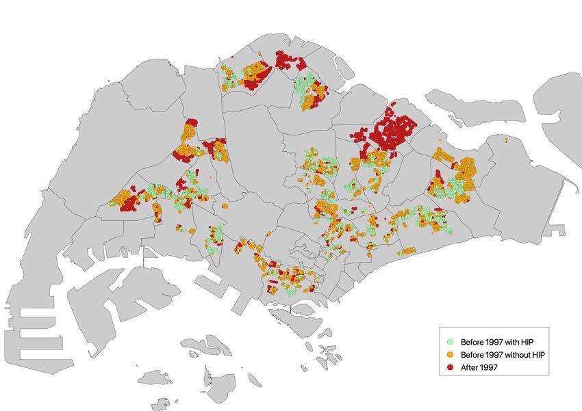
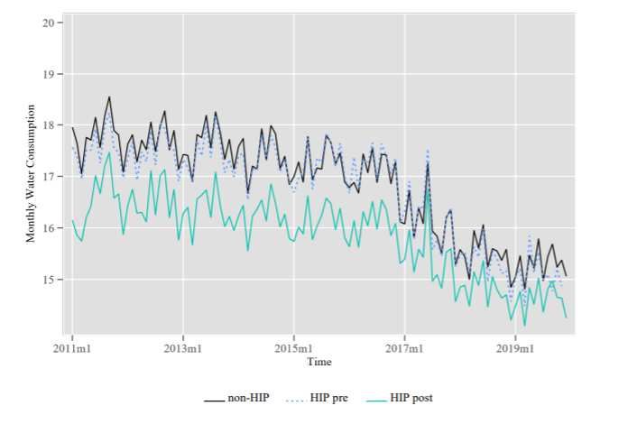
time of upgrading and are likely more efficient than the old installations. The optional

improvements are heavily subsidized with households paying between 5% to 12.5% of the total

cost based upon the flat type (see Supplementary Table B.1). On average, the take-up rate for this

optional upgrade is 70% according to the HDB.

Average intent-to-treat effect

As shown in Figure 1, the mean monthly water consumption for both HIP and non-HIP flats

reduced over time. We observe that the trend for the pre-HIP flats followed closely to that of the

non-HIP flats while the post-HIP water consumption was lower throughout the sample period.

To empirically evaluate the average effect of efficiency improvements on water consumption, we

use a staggered difference-in-differences regression approach comparing the monthly water

consumption for HIP flats before (pre-HIP) and after (post-HIP) project completion, relative to

non-HIP flats. In our empirical estimation, we take into account time-invariant household

characteristics, seasonality, spatial variations in weather and pollution, economy-wide common

shocks as well as group specific pre-trend for HIP and non-HIP flats.

Table 1 column (4) shows the baseline estimate for the average effect of efficiency improvements

on residential water consumption (by estimating equation (1) in Methods). Upon the completion

of HIP, the treated accounts reduced water consumption by 3.5%. Evaluated at the mean monthly

water consumption of 17.24 m3 for HIP flats before project completion, 0.6 m3 of water was saved

per household per month. With approximately 360,000 flats completing the upgrade, annual total

water consumption was estimated to decline by 2,592,000 m3 by December 2019. Note that not all

flats in the treatment group went through the optional bathroom upgrade. As we do not have

 5

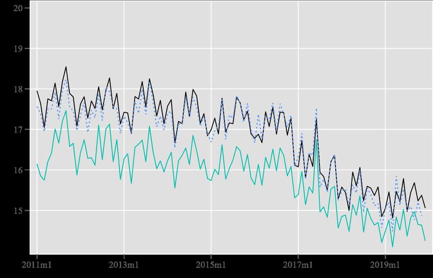
information for the treatment status for each individual flat, this estimate should be considered as

an average intent-to-treat effect.

For robustness checks, we consider (1) alternative cut-off for project completion: instead of using

18 months after polling, we use billing date as the proxy for project completion; (2) alternative

samples: we consider various sample restrictions, including restricting the control groups to flats

of similar age as HIP flats and limit the sample to HIP flats only; (3) alternative clustering for

standard errors. The changes in effect size across models are small, if any (see Supplementary A).

Dynamic effect

In addition to the average treatment effect, we study the long-term and evolutionary effects of

efficiency improvements by conducting an event study (equation (2) in Methods). The coefficients

of this estimation compare the water consumption of HIP flats in each 12-month period before and

after project completion to that of the non-HIP flats.

Figure 2 presents the coefficients with the corresponding 95% confidence intervals where T0 is

the month of project completion taking 18 months after the announcement of HIP polling results

as the cut-off, while T-1 and T+1 refer to the 12 months pre- and post-project completion

respectively. In all time periods before HIP, there was no statistically significant difference in the

mean water consumption for the treatment and control groups, which validates the difference-in-

differences research design. Upon the completion of HIP, there is an immediate reduction in water

consumption for the treatment group. The effect is persistent throughout the sample period, which

covers up to 10 years after HIP completion. Supplementary Figure B.4 presents similar analysis

using alternative samples and the long-term effects are consistent across samples.

 6

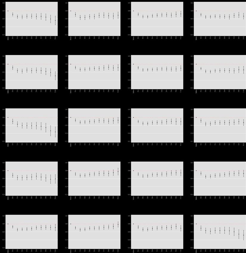
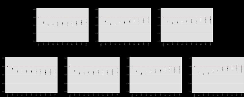
Heterogeneous effect

We next study the heterogeneous effect of efficiency improvements on population subgroups with

varied housing characteristics, water demand and block-level demographics (equation (3) in

Methods). We compare the monthly water consumption for each subgroup of HIP flats before and

after project completion, relative to their counterparts among the non-HIP flats.

Firstly, we investigate the effect of efficiency improvements by housing characteristics such as flat

type and age. As flat types are reflective of income levels, we may observe heterogeneous effect

of HIP on water consumption if the take-up rate for optional upgrades differs across income groups.

Figure 3(a) shows that HIP has a significant effect in reducing water consumption across all flat

types with the effect size for HDB 1-/2-rooms (2.0%) and HDB 5-room/executive flats (3.0%)

smaller than the HDB 3-room (3.5%) and 4-room (3.6%) flats.

Similarly, if the water efficiency of existing fittings in flats built over time improves, we would

observe a decreasing effect of HIP on water consumption. We divide the sample into five time-

windows: before 1980, 1980-1983, 1984-1986, 1987-1997 and after 1997. Flats in the first three

windows qualify for the first phase of HIP and account for 99% of all HIP flats with similar number

of HIP flats in each window. Flats in the fourth window qualify for the second phase of HIP while

the fifth window contains no HIP flats. Figure 3(b) shows, as expected, that the effect of HIP on

residential water consumption to reduce from 3.8% for flats built before 1980, to 3.6% for flats

built between 1980 and 1983 and to 3.1% for flats built between 1984 and 1986.

Next, we divide the sample into water consumption quartiles by the mean water usage for each

account as baseline water demand determines the upper limit of reduction in water consumption

through efficiency improvements. Figure 3(c) shows that, consistent with our hypothesis, HIP

 7

significantly reduces water consumption across all subgroups and the magnitude of reduction

increases from 1.6% for the first quartile, to 3.1%, 3.9% and 4.9% for second, third and fourth

quartile respectively. The trend of increasing effect size as water consumption increases also holds

across subgroups with varied housing characteristics.

Lastly, we evaluate the heterogeneous effect of HIP by block-level demographic characteristics

such as family size, gender, ethnicity and age. As the improvement in water efficiency is not an

intended outcome of the project, we are not expecting immediate behavioural changes that may

differ by demographic characteristics. If HIP does have heterogeneous effects across demographic

groups, it is likely linked to varied baseline water demand. We divide HDB blocks into quartiles

based on their 2011 mean family size, percentage of males, percentage of Chinese, percentage of

elderly, and percentage of young adults. Figure 3(d) to (h) show that the effects of HIP are similar

across subgroups with varied block-level demographic characteristics with few exceptions. For

example, the effect on the lowest quartile of family size is smaller (2.7%). This is consistent with

our previous results as smaller households are likely to have lower water consumption and less

room for reduction.

Supplementary Figure B.5-10 present more details on the subgroup samples and the evolutionary

effects of efficiency improvements by subgroup.

Interaction of HIP and extreme environmental conditions

In our baseline model, we find that a 1% increase in monthly mean temperature (equivalent to 0.28
◦
 C, evaluated at the mean) is associated with a 0.48% increase in water consumption for an average

household. We observe no significant effect of 1% change in the number of rainy days, and PSI

on water consumption. The small effect of a 1% change in weather and pollution on water

 8

consumption is expected because of the limited variation in temperature, rainfall, and air pollution

in Singapore. We therefore focus on how efficiency improvements modify the effect of the extreme

changes in environmental conditions by interacting the indicator variables for extreme temperature,

rainfall and air pollution with the HIP status variables (equation (4) in Methods).

We find that when it is extremely hot (monthly mean temperature above 28.9 ◦C), the monthly

water consumption for an average non-HIP flat increases by 0.7%. The effect on pre-HIP flats is

similar. However, upon project completion, excessive heat no longer has significant effect on

residential water consumption for HIP flats, as illustrated in Figure 4(a).

We also find that excessive rain (more than 22 rainy days in a month) does not affect water

consumption for non-HIP flat; however, it reduces water consumption by 1% for an average pre-

HIP flat. Upon HIP completion, the effect size of excessive number of rainy days reduces and is

no longer statistically significant, as shown in Figure 4(b).

Lastly, when air quality is unhealthy with PSI above 100, the non-HIP and pre-HIP flats are

affected in similar ways with an increase in water consumption by 0.5% and 0.7% respectively.

The completion of HIP makes residential water consumption less susceptible to air pollution with

its effect significantly reduced by 1.1% and no longer statistically significant as shown in Figure

4(c).

The findings in this section suggest that in addition to directly reducing water consumption,

efficiency improvements may also mitigate the effect of extreme weather and air pollution. Results

using alternative model specifications are shown in Supplementary Table B.3 and long-term

effects of the interaction between efficiency improvements and extreme environmental conditions

are presented in Supplementary Figure B.11.
 9

Nation-wide nudging through peer comparison

In the above sections, we show that efficiency improvements through plumbing reduces water

consumption and the effect is persistent up to at least ten years. To put this in perspective, we

evaluate another nation-wide initiative that specifically targets residential water conservation.

In August 2016, the utility bill for residential consumers were redesigned in Singapore. The new

layout of the utility bill allows consumers to view their current and past five months water

consumption. The consumers are also able to compare their own water usage with the average

consumption of their neighbours living in the same flat type within the same block. Additionally,

national average water consumption is provided along with tips on water conservation.

As the bill update was implemented nation-wide, we do not have a suitable control group to clearly

identify the causal effect of peer comparison on residential water consumption. However, for the

peer comparison to work, we would likely observe (1) the mean water consumption for the

comparison groups or block-flat-type groups to reduce; (2) the within block-flat-type group

standard deviation to reduce; (3) more reduction for the accounts that consumes more than the

group mean or the benchmark provided in the newly designed bill. We do not observe any of the

above-mentioned trends through our graphical inspection (as shown in Supplementary Figure

B.12.).

Table 2 shows the empirical estimates on the effect of peer comparison. We restrict the sample

period to November 2016 as a series of other water conservation initiatives were implemented

from December 2016, such as a massive media campaign in December 2016 due to a severe

drought affecting resource availability, and the announcement and implementation of water tariff

increase in February and July 2017.

 10

In columns (1) and (2), we compare the group mean and within group standard deviation in water

consumption before and after the information for peer comparison was made available through

utility bills (equation (5) in Methods). We do not observe any statistically significant reduction in

both outcome variables. In column (3), we compare the water consumption for the accounts that

consumes above the benchmark, or the mean water consumption for the same type of flats within

the same block, before and after the intervention, relative to those who consume below the

benchmark (equation (6) in Methods). We find no statistically different reduction in water

consumption for the two groups.

We investigate the evolutionary effect of peer comparison on all three outcome variables to address

the concern that households may not react immediately to the bill update (equation (7) and (8) in

Methods). We find no trend in the coefficients over time that signals the peer comparison taking

effect slowly (see Supplementary Figure B.13), though we acknowledge the limitation of a short

response period being suitable for evaluation. We also look into the heterogeneous effect of peer

comparison by subgroups of population (equation (9) and (10) in Methods), by flat type, flat age,

and water consumption quartiles, and we are unable to identify any effects across all subgroups

(see Supplementary Figure B.14).

Overall, we are unable to attribute any clear reduction in water consumption to the nation-wide

nudging through redesigned utility bill. Even though the literature has shown a promising local

treatment effect of peer comparison in conservation both globally and in Singapore25, the scale-up

of such interventions may not work based on our results.

 11

Conclusion

In this paper, we show that improving plumbing could obtain long-lasting effects in water

conservation. Using monthly billing data from 1.5 million accounts in Singapore over 10 years,

we show that a nation-wide Home Improvement Programme reduces residential water

consumption by 3.5% on average. Evaluated at the mean before HIP, the program reduces monthly

water consumption by 0.6 cubic meters per household on average. Although the savings on water

tariff alone are not able to recover the upfront cost at the household level, we should note that

efficiency improvements is not the main focus of the program, yet it provides additional benefits

to the upgrade and results in larger water savings than a national-wide behavioural nudging. As

Singapore aims to reduce residential water consumption from 141 litres per person per day in 2018

to 130 litres in 2030, our back-of-the-envelope estimation show that the 3.5% water savings could

potentially contribute to half of this conservation target for the HIP households.

We find that the effect of efficiency improvements on water consumption last at least a decade, in

contrary to the short-term effect of behavioural nudging. In terms of policy design, efficiency

improvements is more straightforward, unlike behavioural interventions that require careful

calibrations to ensure effectiveness. We also show that the effect of efficiency improvements is

observed across population subgroups. It helps in mitigating the effect of extreme environmental

conditions on water use. Nation-wide nudging through peer comparison, however, may not achieve

similar outcomes.

There are a few caveats in our findings on the effectiveness of efficiency improvements. Firstly,

we are unable to control for time-varying household characteristics due to lack of data. It is

possible that time-variant changes in household characteristics may affect the accuracy of our

 12

estimates. However, it is unlikely that the average changes in household characteristics for the

treatment group would differ from that of the control group given the exogenous selection into the

program and the fact that our data covers 80% of the total population in the country. Secondly, we

do not have information on the specifications of water fittings before or after HIP. The efficiency

improvements and the estimated effect are based on technological advances in the water fittings

over time. Thirdly, apart for the overall take-up rate of 70%, we do not have information on the

exact households that opted in vs out of the optional bathroom upgrade, therefore we are only able

to estimate the intent-to-treat effect of the efficiency improvements.

This paper contributes to the literature by showing for the first-time robust empirical evidence that

(1) improving plumbing can obtain long-lasting effects on water conservation; (2) efficiency

improvements helps in mitigating the effect of extreme weather and environmental conditions on

water use; and (3) nation-wide nudging through peer comparison may not achieve similar

outcomes.

Methods

Data

Water consumption: We use water consumption data obtained from PUB, Singapore’s national

water agency. It contains monthly water consumption based on water bills for all HDB flats with

1,506,296 unique anonymized accounts from January 2011 to December 2019. The data includes

anonymized account number that changes every time a household moves, block identifier/postal

code, and flat type classified by the number of rooms.

Block-level housing characteristics and demographics: Housing characteristics such as year of

completion were collected through publicly available database provided by the Government of

 13

Singapore. Additionally, we have access to administrative data on the demographics and

residential addresses for 2.8 million adult Singaporeans in 2011. Although we are unable to match

these individuals to account level water consumption due to the anonymization of premise

identifier in the water consumption data, we could derive block-level demographics, such as mean

family size, percentage of males (vs. female), percentage of Chinese (vs. other ethnicity),

percentage of elderly (born before 1950) and percentage of young adults (born after 1990).

Weather and air quality: We acquire daily weather observations by station from the Meteorological

Service Singapore and historical 24-hour Pollutant Standards Index (PSI) readings by monitor

from the National Environmental Agency. We generate block-specific monthly weather and air

quality indicators such as mean temperature, number of rainy days, and mean PSI using

observations across all stations within 10-kilometer (km) radius of the block using Inverse

Distance Weighting method. The trend and spatial variations over time are shown in

Supplementary Figure B.3.

Sample: In our baseline analysis, we include sample from January 2011 to December 2019. We

exclude extreme values of the top and bottom 1% observations in water consumption for each flat

type to account for potential measurement errors caused by water leakage, bill adjustment, and

problematic meter readings. We exclude accounts with missing information on HIP status. The

resulting baseline sample consists of 98,291,320 observations from 1,503,350 accounts in 10,188

HDB blocks.

Sample statistics are shown in Supplementary Table B.2. The mean monthly water consumption

is 17.24 m3 for HIP flats before project completion, higher than 16.8 m3 for non-HIP flats; while

the post-project mean for HIP flats is reduced to 15.42 m3.

 14

The treatment and control groups comprise a different mix of flats in terms of year of construction

and flat type. This is expected as only older flats built before 1997 were eligible for HIP and the

composition of flat types evolved over time to accommodate the changing demographics. Similarly,

we observe differences in demographic composition between HIP and non-HIP flats. During the

sample period, the differences in weather and air quality between treatment and control groups

were small.

Empirical method

Effect of efficiency improvements

We analyse the effect of efficiency improvements on residential water consumption using a

staggered difference-in-differences regression approach. The treatment group is the HDB flats that

completed HIP before December 2019, and the control group is the HDB flats that did not

implement or complete the project. We use sample from January 2011 to December 2019 therefore

the pre-treatment time-periods range from 1 to 107 months while the post-treatment periods range

from 1 to 124 months due to the staggered implementation of HIP.

To evaluate the average effect of efficiency improvements on water consumption, we first estimate

the following equation:

 ln = × + + + + + 
 (1)

The dependent variable is the natural logarithm of monthly water consumption for household i

living in block j in time period t. Postt is an indicator variable that takes the value of 1 for time

periods post the completion of HIP. Treati is an indicator variable for the treatment group, that is,

household that completed HIP. Xjt is a vector of weather and air quality controls such as the log of
 15

mean temperature, number of rainy days, and mean PSI, which vary by block and time. We allow

the control and treatment groups to have different water consumption trends by including group-

specific linear time trend τ. We include household fixed effects αi to account for time-invariant

household characteristics and time fixed effect γt to account for seasonality and other economy-

wide common shocks. The coefficient of interest δ measures the average post-completion monthly

water consumption for the treatment group relative to the control group. Standard errors in the

baseline estimation are two-way clustered by block and year-month.

We further explore the dynamics of water consumption change due to efficiency improvements

through an event study analysis and estimate the following model:

 10
 
 ln = � × + + + + + 
 =−9
 (2)

where we interact the treatment indicator with a set of relative time dummies Dityear that correspond

to each 12-month lead and lag of the treatment timing. In our sample, the data covers observations

up to 9 years before and 10 years after the HIP implementation. The coefficients of interest δl

measure the average difference in water consumption between the control and treatment group in

each 12-month period. In addition, this setting also allows us to explicitly test the parallel trend

assumption of the difference-in-differences design.

We study the heterogeneous effect of efficiency improvements on subgroups of population by

housing characteristics (i.e. by flat type, flat age categories), water demand (i.e. water consumption

quartile), and block-level demographic characteristics (i.e. quartile of family size, percentage of

 16

males, percentage of Chinese, percentage of elderly and percentage of young family), using the

following specification:

 ln = � × × + + + + + 
 =1
 (3)

where N is the number of subgroups and Gi is the subgroup indicator. The coefficients δ1 to δN

measure the heterogeneous effect of efficiency improvements.

We are particularly interested in whether efficiency improvements modify the effect of

environmental conditions. To this end, we estimate the interaction effect between weather/air

quality variables and HIP through the following equation:

 ln = × + 1 + 2 × + 3 × + + + + + 
 (4)

where Xjt is a weather or pollution control variable for all households in block j during time t. The

coefficients β1, β1 + β2 and β1 + β2 + β3 represent the effect of weather and pollution on non-HIP

flats, HIP flats before and after project completion, respectively.

Effect of peer comparison

Firstly, we expect peer comparison to reduce both the mean water consumption and within block-

flat-type standard deviation. To test this, we estimate the following equation:

 ln = + + + + ℎ + 
 (5)

 17

Where Yjt is the mean or standard deviation of water consumption for block-flat-type j in month t;

Postt is and indicator variable that takes the value of 1 for time periods after the bill update; Xjt is

a vector of weather and air quality controls such as the log of mean temperature, number of rainy

days, and mean PSI, which vary by block and time. We include group fixed effects αj to account

for time-invariant group characteristics; month fixed effects ℎ to account for seasonality; and

year fixed effects to account for common economy-wide shocks each year.

Secondly, for the peer comparison to work, we would expect more reduction for the accounts that

consume more than the group mean or the benchmark provided in the newly designed bill. We

divide the accounts into two groups based upon pre-treatment mean water consumption. We

compare water consumption before and after bill update for the above-the-mean group, relative to

that of the blow-the-mean group by estimating the following equation:

 ln = × + + + + 
 (6)

Where Wit is the water consumption for account i in time period t; Abovei is an indicator variable

for the above-the-mean group; α and γ are account fixed effects and year-month fixed effects

respectively.

We estimate the evolutionary and heterogeneous effect of peer comparison for the three outcome

variables of concern through the following equations:

 4

 ln = � + + + + ℎ + 
 =1
 (7)
 4

 ln = � × + + + + 
 =1
 (8)
 18

 

 ln = � × + + + + ℎ + 
 =1
 (9)
 
 ln = � × × + + + + 
 =1
 (10)

where D is the time dummies for each of the post bill update month and G is sub-groups dummies.

Data availability statement

The data for this study is provided PUB, Singapore's National Water Agency under non-
disclosure agreement for the current study and is not publicly available. However, it may be
obtained with data use agreement with the PUB.

Code availability statement

Stata code for data cleaning and analysis will be made available upon request.

 19

References

1. Hunt Allcott. Social norms and energy conservation. Journal of Public Economics, 95(9-
 10):1082–1095, oct 2011.
2. Daniel A. Brent, Joseph H. Cook, and Skylar Olsen. Social comparisons, household water use,
 and participation in utility conservation programs: Evidence from three randomized trials.
 Journal of the Association of Environmental and Resource Economists, 2(4):597–627, dec
 2015.
3. Paul J Ferraro, Juan Jose Miranda, and Michael K Price. The persistence of treatment effects
 with norm-based policy instruments: Evidence from a randomized environmental policy
 experiment. American Economic Review, 101(3):318–322, may 2011.
4. Paul J. Ferraro and Michael K. Price. Using nonpecuniary strategies to influence behavior:
 Evidence from a large-scale field experiment. Review of Economics and Statistics, 95(1):64–
 73, mar 2013.
5. Hunt Allcott and Todd Rogers. The short-run and long-run effects of behavioral interventions:
 Experimental evidence from energy conservation. American Economic Review, 104(10):3003–
 3037, oct 2014.
6. Mark A. Andor and Katja M. Fels. Behavioral economics and energy conservation – a
 systematic review of non-price interventions and their causal effects. Ecological Economics,
 148:178–210, jun 2018.
7. Richard G. Newell and Juha Siikamäki. Nudging energy efficiency behavior: The role of
 information labels. Journal of the Association of Environmental and Resource Economists,
 1(4):555–598, dec 2014.
8. Ben Gilbert and Joshua Graff Zivin. Dynamic salience with intermittent billing: Evidence from
 smart electricity meters. Journal of Economic Behavior & Organization, 107:176–190, nov
 2014.
9. Katrina Jessoe and David Rapson. Knowledge is (less) power: Experimental evidence from
 residential energy use. American Economic Review, 104(4):1417–1438, apr 2014.
10. Casey J. Wichman. Information provision and consumer behavior: A natural experiment in
 billing frequency. Journal of Public Economics, 152:13–33, aug 2017.
11. Dora L. Costa and Matthew E. Kahn. Energy conservation “nudges” and environmentalist
 ideology: Evidence from a randomized residential electricity field experiment. Journal of the
 European Economic Association, 11(3):680–702, jun 2013.
12. Hunt Allcott and Judd B. Kessler. The welfare effects of nudges: A case study of energy use
 social comparisons. American Economic Journal: Applied Economics, 11(1):236– 276, jan
 2019.
13. Hunt Allcott and Michael Greenstone. Is there an energy efficiency gap? Journal of Economic
 Perspectives, 26(1):3–28, feb 2012.

 20

14. Kenneth Gillingham, Amelia Keyes, and Karen Palmer. Advances in evaluating energy
 efficiency policies and programs. Annual Review of Resource Economics, 10(1):511–532, oct
 2018.
15. Joshua Graff Zivin and Kevin Novan. Upgrading efficiency and behavior: Electricity savings
 from residential weatherization programs. The Energy Journal, 37(4), 2016.
16. Hunt Allcott and Michael Greenstone. Measuring the welfare effects of residential energy
 efficiency programs. Technical report, NBER Working Papers 23386., 2017.
17. Meredith Fowlie, Michael Greenstone, and Catherine Wolfram. Do energy efficiency
 investments deliver? evidence from the weatherization assistance program. The Quarterly
 Journal of Economics, 133(3):1597–1644, jan 2018.
18. Jing Liang, Yueming Qiu, Timothy James, Benjamin L. Ruddell, Michael Dalrymple, Stevan
 Earl, and Alex Castelazo. Do energy retrofits work? evidence from commercial and residential
 buildings in phoenix. Journal of Environmental Economics and Management, 92:726–743,
 nov 2018.
19. Lucas W. Davis, Alan Fuchs, and Paul Gertler. Cash for coolers: Evaluating a largescale
 appliance replacement program in Mexico. American Economic Journal: Economic Policy,
 6(4):207–238, nov 2014.
20. Grant D. Jacobsen and Matthew J. Kotchen. Are building codes effective at saving energy?
 evidence from residential billing data in Florida. The Review of Economics and Statistics,
 95(1):34–49, March 2013.
21. Arik Levinson. How much energy do building energy codes save? evidence from California
 houses. American Economic Review, 106(10):2867–2894, oct 2016.
22. Yueming Qiu and Matthew E. Kahn. Better sustainability assessment of green buildings with
 high-frequency data. Nature Sustainability, 1(11):642–649, nov 2018.
23. Kevin Novan, Aaron Smith, and Tianxia Zhou. Residential building codes do save energy:
 Evidence from hourly smart-meter data. The Review of Economics and Statistics, pages 1–45,
 sep 2020.
24. Matthew J. Kotchen. Longer-run evidence on whether building energy codes reduce residential
 energy consumption. Journal of the Association of Environmental and Resource Economists,
 4(1):135–153, mar 2017.
25. Sumit Agarwal, Satyanarain Rengarajan, Tien Foo Sing, and Yang Yang. Nudges from school
 children and electricity conservation: Evidence from the “project carbon zero” campaign in
 Singapore. Energy Economics, 61:29–41, jan 2017.

 21

Acknowledgements

All the authors acknowledge the funding and water consumption data support from the PUB,

Singapore’s National Water Agency.

Contribution

All authors contributed to the research design, implementation, data analysis and writing.

Conflicts of interests

None of the authors have any conflicts of interests.

 22

Figures and Tables

 Figure 1: Trend of monthly water consumption

 non-HIP HIP pre HIP post

Note: The figure shows the trend in monthly mean water consumption (in cubic meter) for non-HIP flats,
HIP flats before HIP completion, HIP flats after HIP completion over time.

 23

Figure 2: Evolutionary effect of HIP on water consumption

Note: The figure shows the coefficients and corresponding 95% confidence intervals for the difference in
water consumption between flats that completed and did not complete HIP each year before and after HIP
completion by estimating equation (3).

 24

Figure 3: Heterogeneous effect by housing characteristics, water demand and block-level demographics
 0.02 0.02 0.02

 0.00 0.00 0.00

 -0.02
 -0.02 -0.02

 -0.04
 -0.04 -0.04

 -0.06
 -0.06 -0.06
 Quartile 1 Quartile 2 Quartile 3 Quartile 4
 1-/2-room 3-room 4-room 5-room/Executive Before 1980 1980-1983 1984-1986 1987-1997 (0-9.05] (9.05 , 14.7] (14.7 , 21.5] (21.5 , 66.5]

 (a) By flat type (b) By year of construction (c) By water consumption quartile

Note: The figures show the coefficients and corresponding 95% confidence intervals for the effect of HIP on monthly water consumption for each
subgroup by estimating equation (4). Sub-figures (a), (b) and (c) show the effects by flat type, year of construction, and water consumption
quartile, respectively. Sub-figures (d) to (h) present the heterogeneous effects by quartiles of family size, percentage of male, percentage of
Chinese, percentage of elderly and percentage of young family.

Figure 4: Effect of extreme environmental conditions on HIP vs non-HIP flats
 0.02

 0.01

 0.00

 -0.01

 -0.02
 Non-HIP HIP pre HIP post

 (a) Temperature
 0.02

 0.01

 0.00

 -0.01

 -0.02
 Non-HIP HIP pre HIP post

 (b) Number of rainy days
 0.02

 0.01

 0.00

 -0.01

 -0.02
 Non-HIP HIP pre HIP post

 (c) PSI

Note: The figures show the coefficients and corresponding 95% confidence intervals for the effect of high
temperature, excessive number of rainy days and high PSI on non-HIP flats (β1), HIP flats before (β1 + β2)
and after (β1 + β2 + β3) project completion, by estimating equation (5). To be more specific, the coefficients
in Panels (a), (b) and (c) correspond to Table A.2.3 column (5) row 2, row 2+5, and row 2+5+6; column (6)
row 3, row 3+7, and row 3+7+8; and column (7) row 4, row 4+9, and row 4+9+10, respectively.

 26

Table 1: Average intent-to-treat effect of HIP on water consumption

 (1) (2) (3) (4)

 Dependent variable: Log of water consumption

 HIP*Completed -0.035*** -0.035*** -0.035*** -0.035***
 (0.002) (0.002) (0.002) (0.002)
 Weather control Yes Yes No Yes
 Pollution control Yes Yes No Yes
 Group time trend Yes Yes Yes Yes
 Account FE No Yes Yes Yes
 Block FE Yes No No No
 Year-month FE Yes No Yes Yes
 Year FE No Yes No No
 Month FE No Yes No No
 N 98,291,320 98,291,320 98,291,320 98,291,320
 2 0.108 0.740 0.740 0.740
 R
Note: This table presents the average intent-to-treat effect of HIP on water consumption for the treatment
group post project completion, relative to the control group. The dependent variable is log of monthly water
consumption. HIP is an indicator variable that takes the value of 1 for the treatment group; Completed is
an indicator variable that takes the value of 1 for time periods post project completion. Column (4) shows
the baseline estimates, by estimating equation (2). Column (1) alter the baseline estimation by including
block fixed effects instead of account fixed effects; column (2) includes year fixed effects and month fixed
effects instead of year-month fixed effects; column (3) does not include weather and pollution controls. The
standard errors shown in parentheses are clustered by block and year-month. * p < 0.1, ** p < 0.05, *** p
< 0.01.

 27

Table 2: Effect of peer comparison on water consumption

 (1) (2) (3)
 Dependent variable: Log of group mean Log of within group sd Log of water consum.
 Post bill update -0.005 0.004
 (0.006) (0.005)
 Post bill update*Above mean -0.001
 (0.010)
 Control Yes Yes Yes
 Account FE No No Yes
 Block by flat-type FE Yes Yes No
 Year-month FE No No Yes
 Year FE Yes Yes No
 Month FE Yes Yes No
 N 500,993 500,993 28,307,707
 R2 0.856 0.660 0.807
Note: The table presents the effect of peer comparison on water consumption. Columns (1) and (2) compare
the group mean water consumption and within group standard deviation before and after the bill update,
where each flat type within an HDB block constitutes a comparison group. Column (3) compares monthly
water consumption for accounts that consumes above the group mean before and after the bill update,
relative to the accounts that consumes below the group mean. All models include weather and pollution
controls. Columns (1) and (2) in both Panels include block by flat-type fixed effects, year fixed effects and
month fixed effect. Column (3) includes account fixed effects and year-month fixed effects. The standard
errors are two-way clustered by block and year-month. * p < 0.1, ** p < 0.05, *** p < 0.01. Standard error
in parenthese

 28

Supplementary information
A. Robustness checks on the average effect of efficiency improvements
For robustness checks, we consider (1) alternative cut-off for project completion; (2) alternative
samples; (3) alternative clustering for standard errors.

As the exact timing of project completion for each flat is unknown, we use 18-month post the
announcement of a successful poll as a proxy in our baseline analysis. Using a more conservative
cut-off, time of billing, we find a similar (3.4%) reduction in water consumption for the treatment
group as shown in Table A.1 column (2). Note that it could take up to two years from the time of
project completion to the time a household receives the bill, hence the estimated effect size using
the time of billing as the cut-off is expected to be smaller.

In our baseline analysis, we use all flats that did not implement or complete HIP as the control
group. However, there may be a concern that HDB flats built during different times have inherent
differences in their characteristics, leading to biased estimates on the effect of HIP. To address this
concern, we restrict the sample step-by-step based upon the year of construction of the HDB flats
and re-estimate equation (1) using these alternative samples. The estimates are shown in Table A.3
columns (2) to (6). First, we restrict the sample to HDB flats built before 2008. In 2008, the
Mandatory Water Efficiency Labelling Scheme was introduced and the HDB flats built after 2008
were required to comply with this standard and may differ in their water efficiency level. If this is
the case, including flats built after 2008 as part of the control group would lead to over-estimation
of the effect of HIP; however, as shown in Table A.3 column (2), the estimate using the restricted
sample does not differ from our baseline estimate. Second, we restrict the sample to the flats that
qualify for the first (built before 1986) and second (built before 1997) phase of HIP, respectively.
This is to eliminate the concern that the HIP eligibility cut-off may be correlated with water
efficiency levels of HDB flats, although this is not likely the case since efficiency improvements
was not the primary aim of HIP. As shown in Table A.3 columns (3) and (4), the estimates using
samples restricted to flats built before 1997 and 1986 are 3.3%, only marginally lower than that of
the baseline estimate. Third, we further exclude HDB flats built before 1970 to avoid the effect of
HIP being skewed by really old flats with potentially extreme efficiency gains. As shown in Table
A.3 column (5), the estimated effect remains as 3.3%. Last, we restrict the sample to flats built in

 29

1986 and 1987 only or just around the eligibility cut-off for the first phase of HIP. This is to ensure
that HIP is the main differentiating factor between the treatment and control group while other
sample characteristics are similar. The normalized differences between the treatment and control
groups for each alternative sample are presented in Table A.2. We observe in Table A.3 column
(6) that the estimate is 3.0%, slightly lower than that of the baseline sample.

For the remaining concern that the flats that completed HIP may have different characteristics or
pre-HIP water efficiency level as compared to the ones that did not implement or complete HIP,
we restrict our sample to HIP flats only. Exploiting the variation caused by the staggered timing
of HIP completion, we estimate the effect of HIP on residential water consumption to be 3.3%, as
shown in Table A.3 column (7).

As an additional robustness check, we relax the sample restriction by including the top and bottom
1% observations in monthly water consumption in our sample. As shown in Table A.3 column (8),
there is only a slight increase in the effect size from 3.5% in the baseline sample to 3.7% in the
alternative sample without restriction on extreme values.

Standard errors in the baseline estimation are two-way clustered by block and year-month. Results
using alternative clustering methods are included in Table A.4.

 30

Table A.1: Effect of HIP on water consumption using alternative cut-off for project completion

 (1) (2)

 Dependent variable: Log of water consumption

 HIP*Completed -0.035***
 (0.002)
 HIP*Billed -0.034***
 (0.002)
 Weather control Yes Yes
 Pollution control Yes Yes
 Group time trend Yes Yes
 Account FE Yes Yes
 Year-month FE Yes Yes
 N 98,291,320 98,291,320
 2
 R 0.740 0.740
Note: This table presents the average intent-to-treat effect of HIP on water consumption for the treatment
group post project completion, relative to the control group, using alternative cut-off for project completion.
The dependent variable is log of monthly water consumption. HIP is an indicator variable that takes the
value of 1 for the treatment group; Completed is an indicator variable that takes the value of 1 for time
periods post project completion; Billed is an indicator variable that takes the value of 1 for time periods
post billing. Column (1) shows the baseline estimates and column (2) uses billing date as an alternative cut-
off for project completion. All models include weather and pollution controls, group specific linear time
trend, account fixed effects and year-month fixed effects. The standard errors shown in parentheses are
two-way clustered by block and year-month. * p < 0.1, ** p < 0.05, *** p < 0.01.

 31

Table A.2: Normalized difference in descriptive statistics for alternative samples

 (1) (2) (3) (4) (5)
 ≤2008 ≤1997 ≤1986 1971-86 1986-87

 Panel A: Water consumption
 Mean before HIP (m3) 0.02 0.01 -0.18 -0.13 -0.01
 Panel B: Characteristics
 Year of construction
 Before 1980 -0.12 0.07 0.85 0.66
 1980-1983 -0.70 -0.64 -0.46 -0.39

 1984-1986 -0.89 -0.79 -0.48 -0.35

 1987-1997 1.06 1.42

 After 1997 0.86

 Flat type
 1-/2-room 0.27 0.34 0.59 0.47 0.60
 3-room -0.58 -0.42 0.05 -0.02 -0.05
 4-room -0.02 -0.06 -0.33 -0.21 0.18
 5-room and Executive 0.47 0.35 -0.11 -0.02 -0.15
 Demographics
 Mean family size -0.07 -0.05 -0.15 -0.07 0.01
 Mean prop. of males 0.114 0.07 -0.16 0.06 0.12
 Mean prop. of Chinese 0.05 -0.05 0.03 0.01 -0.16
 Mean prop. of elderly -0.45 -0.22 0.78 0.59 -0.06
 Mean prop. of young adults 0.12 -0.24 -0.27 -0.22 0.10
 Weather and pollution
 Mean temperature (C◦) -0.03 -0.02 0.07 0.06 0.07
 Mean no. of rainy days 0.01 0.00 -0.02 -0.01 -0.02
 Mean PSI 0.00 0.00 0.00 0.00 0.00
 Observations 86,732,067 69,771,942 46,002,072 41,526,217 6,500,267
Note: This table presents the normalized difference in the group mean for HIP and non-HIP flats for
alternative samples. Columns (1) to (5) use HDB flats built before 2008; HDB flats built before 1997 or
qualifies for HIP; HDB flats built before 1986 or qualifies for the first phase of HIP; HDB flats built
between 1971 to 1986; and HDB flats built in 1986/87 or around the cut-off for the first phase, respectively.

 32

Table A.3: Effect of HIP on water consumption using alternative samples

 Dependent variable: (1) (2) (3) (4) (5) (6) (7) (8)
 Log of water consumption Baseline ≤2008 ≤1997 ≤1986 1971-86 1986-87 HIP only w/ extremes

 -
 HIP*Completed -0.035*** -0.035*** -0.033*** -0.033*** -0.033*** 0.030*** -0.033*** -0.037***
 (0.002) (0.002) (0.002) (0.002) (0.001) (0.002) (0.002) (0.002)

 Weather control Yes Yes Yes Yes Yes Yes Yes Yes
 Pollution control Yes Yes Yes Yes Yes Yes Yes Yes
 Group time trend Yes Yes Yes Yes Yes Yes No Yes
 Account FE Yes Yes Yes Yes Yes Yes Yes Yes
 Year-month FE Yes Yes Yes Yes Yes Yes Yes Yes
 N 98,291,320 86,732,067 69,771,942 46,002,072 41,526,217 6,500,267 24,655,772 99,859,740
 2
 R 0.74 0.74 0.753 0.752 0.752 0.748 0.749 0.717
Note: This table presents the average intent-to-treat effect of HIP on water consumption for the treatment group post project completion, relative to
the control group, using alternative samples. The dependent variable is log of monthly water consumption. HIP is an indicator variable that takes
the value of 1 for the treatment group; Completed is an indicator variable that takes the value of 1 for time periods post project completion.
Column (1) shows the baseline estimates using the full sample; column (2) uses HDB flats built before 2008 when Mandatory Water Efficiency
Standards was implemented; column (3) uses HDB flats built before 1997 or qualifies for HIP; column (4) uses HDB flats built before 1986 or
qualifies for the first phase of HIP; column (5) uses HDB flats built between 1971 to 1986 to exclude very old flats; column (6) uses flats built in
1986/87 or around the cut-off for the first phase; column (7) uses only HDB flats that has completed HIP; column (8) removes the restriction on
baseline sample by including the top and bottom 1% observation in monthly water consumption. All models include weather and pollution
controls, group specific linear time trend, account fixed effects and year-month fixed effects. The standard errors shown in parentheses are two-
way clustered by block and year-month. * p < 0.1, ** p < 0.05, *** p < 0.01.

Table A.4: Alternative clustering

 Dependent variable: (1) (2) (3) (4)
 Log of water consumption Two-way One-way
 Account,Year-month Block,Year-month Account Block

 HIP*Completed -0.035*** -0.035*** -0.035*** -0.035***
 (0.002) (0.002) (0.001) (0.001)

 Weather control Yes Yes Yes Yes
 Pollution control Yes Yes Yes Yes
 Group time trend Yes Yes Yes Yes
 Account FE Yes Yes Yes Yes
 Year-month FE Yes Yes Yes Yes
 N 98,291,320 98,291,320 98,291,320 98,291,320
 2
 R 0.740 0.740 0.740 0.740
Note: This table presents the average effect of HIP on water consumption with alternative clustering for
standard error. The dependent variable is log of monthly water consumption. HIP is an indicator variable
that takes the value of 1 for the treatment group; Completed is an indicator variable that takes the value of
1 for time periods post project completion. Standard errors are two-way clustered by account and year-
month for column (1), and by block and year-month for column (2); they are one-way clustered by account
for column (3) and by block for column (4). All models include weather and pollution controls, group
specific linear time trend, account fixed effects and year-month fixed effects. * p < 0.1, ** p < 0.05, *** p
< 0.01. Standard error in parentheses.

 34

B. Additional figures and tables

 Figure B.1: Map of HDB blocks by HIP status

Note: The map shows the location of all HDB blocks in Singapore. The green circles represent HDB blocks
that completed HIP by December 2019; the yellow circles represent HDB blocks that qualifies (i.e. built
before 1997) for HIP but did not go through or complete the upgrade by December 2019; the red circles
represent HDB blocks that do not qualify for HIP (i.e. built after 1997).

 35

Figure B.2: Distribution of HDB flats by year of HIP completion

 100000

 80000

 60000

 40000

 20000

 0
 2009 2010 2011 2012 2013 2014 2015 2016 2017 2018 2019

 Central East North North-east West

Note: The figure shows the number of HDB flats in each region (Central, East, North, Northeast, and West)
by year of HIP completion. Projects are considered complete 18 months after the announcement of a
successful poll. from the Government of Singapore.

 36

Figure B.3: Trend and spatial variation in temperature, rainfall, and air pollution
 Mean temperature Standard deviation of mean temperature
 30 .8

 29
 .6

 28

 .4

 27

 .2
 26

 25 0
 2011m1 2013m1 2015m1 2017m1 2019m1 2011m1 2013m1 2015m1 2017m1 2019m1

 (a) Mean and standard deviation in temperature

 Mean number of rainy days Standard deviation of number of rainy days
 30 4

 25

 3

 20

 15 2

 10

 1

 5

 0 0
 2011m1 2013m1 2015m1 2017m1 2019m1 2011m1 2013m1 2015m1 2017m1 2019m1

 (b) Mean and standard deviation in number of rainy days

 Mean PSI Standard deviation of PSI
 120 5

 100
 4

 80
 3

 60

 2
 40

 1
 20

 (c) Mean and standard deviation in PSI

Note: The figures show the trend and spatial variation (in terms of standard deviation) in monthly mean
temperature (Panel (a)), number of rainy days (Panel (b)), and PSI (Panel (c)) from January 2011 to
December 2019.

 37

Figure B.4: Evolutionary effect of HIP using alternative samples

 (a) Before 2008 (b) Before 1997

 (c) Before 1986 (d) 1971-1986

 (e) 1986-1987 (f) HIP flats only

Note: The figures show, for each alternative sample, the coefficients and corresponding 95% confidence
intervals for the difference in water consumption between flats that completed and did not complete HIP
for each 12-month period after HIP completion. Sub-figures (a) to (f) use HDB flats built before 2008;
HDB flats built before 1997 or qualifies for HIP; HDB flats built before 1986 or qualifies for the first phase
of HIP; HDB flats built between 1971 to 1986; HDB flats built in 1986/87 or around the cut-off for the first
phase; and HDB flats that has completed HIP only, respectively.

 38

Figure B.5: Number of observations by housing characteristics and water demand
 30000000

 20000000

 10000000

 0
 Non-HIP HIP Non-HIP HIP Non-HIP HIP Non-HIP HIP

 HDB 1-/2-room HDB 3-room HDB 4-room HDB 5-room/Executive

 (a) By flat type
 25000000

 20000000

 15000000

 10000000

 5000000

 0
 Non-HIP HIP Non-HIP HIP Non-HIP HIP Non-HIP HIP Non-HIP HIP

 Before 1980 1980-1983 1984-1986 1987-1997 After 1997

 (b) By year of construction
 20000000

 15000000

 10000000

 5000000

 0
 Non-HIP HIP Non-HIP HIP Non-HIP HIP Non-HIP HIP

 Quartile 1 Quartile 2 Quartile 3 Quartile 4

 (c) By water consumption quartile

Note: The figures show the number of observations for treatment and control groups by flat type (Panel
(a)), year of construction (Panel (b)) and water consumption quartile (Pane (c)).

 39

Figure B.6: Sample distribution by water consumption quartile and housing characteristics
 100

 80

 60

 40

 20

 0
 1-/2-room 3- room 4-room 5-room/Executive

 Quartile 1 Quartile 2 Quartile 3 Quartile 4

 (a) By flat type
 100

 80

 60

 40

 20

 0
 Before 1980 1980-1983 1984-1986 1987-1997 After 1997

 Quartile 1 Quartile 2 Quartile 3 Quartile 4

 (b) By year of construction

Note: The figure shows the proportion of observations for each water consumption quartile by flat type
(Panel (a)) and year of construction (Panel (b)).

 40