Economic and Jobs Impacts of Enhanced Fuel Efficiency Standards for Light Duty Vehicles in
←
→
Page content transcription
If your browser does not render page correctly, please read the page content below
ISSN: 2277-3754
ISO 9001:2008 Certified
International Journal of Engineering and Innovative Technology (IJEIT)
Volume 4, Issue 7, January 2015
Economic and Jobs Impacts of Enhanced Fuel
Efficiency Standards for Light Duty Vehicles in the
USA
Roger H. Bezdek, MISI, Robert M. Wendling, MISI
would be consistent with the Environmental Protection
Abstract: This paper estimates the economic impacts of Agency’s and NHTSA’s respective statutory authorities,
strengthening fuel economy and greenhouse gas (GHG) in order to continue to guide the automotive sector along
emission standards for passenger vehicles in the USA, and our the road to reducing its fuel consumption and GHG
research coincides with implementation of new fuel economy emissions.3
and GHG emission standards for passenger vehicles for 2017-
2025. We find that enhanced standards -- more miles and
The policy landscape has also been influenced by key
fewer emissions per gallon -- would lead to increased U.S. legal rulings, including a Supreme Court decision, 4
economic and job growth, both within the auto industry and finding that GHGs are pollutants under the Clean Air Act
throughout the economy. We analyze the impacts of the and subject to regulation by EPA, and district court cases
different regulatory scenarios considered, and find that upholding the right of California to adopt vehicle GHG
positive economic and jobs impacts will result from higher standards and that of states to adopt California’s
standards, and will be more pronounced as standards
strengthen. Economic and jobs impact estimates are made for
standards.5 In May 2009, the U.S. announced the first
the year 2030 for each of the four alternative standards national policy governing both fuel economy and GHG
considered by the U.S. government. Consumer savings and emissions standards for cars and light trucks for model
GHG reductions from the alternative standards are estimated, years 2012-2016. This program grew out an agreement
and economic and jobs impacts are disaggregated by industry between the automakers, California, and the Obama
and by state. Administration, the Environmental Protection Agency
Key Words: Vehicle fuel efficiency, CAFE standards,
(EPA) and NHTSA. Finalized on April 1, 2010, the rule
greenhouse gas emissions, economic impact, jobs impact. requires that fleet averaged fuel economy reach an
equivalent of 34.1 mpg and 250 grams of CO2 per mile by
model year 2016.6
I. INTRODUCTION In June 2011, the U.S. announced new performance
The impacts of fuel consumption by light duty vehicles standards equivalent to 54.5 mpg or 163 grams/mile of
(LDVs) are significant, and the rapid rise in gasoline and CO2 for cars and light-duty trucks by MY 2025, with
diesel fuel prices experienced in recent years, in implementation being phased in beginning with MY
conjunction with concerns over greenhouse gas (GHG) 2017.7 Since LDVs account for more than 40 percent of
emissions from mobile sources, have made vehicle fuel U.S. oil consumption, and nearly 60 percent of mobile
economy an important policy issue. U.S. corporate source GHGs,8 the new standards have important
average fuel economy (CAFE) standards have saved implications for U.S. transportation policy, energy
substantial amounts of petroleum and have played an security, oil consumption and imports, and GHG
important role in reducing vehicle GHG emissions. emissions.
However, until recently, revision of the CAFE standards Credible analysis and data are required to assess the
has been blocked, in part, by concerns over the economic energy, economic, and job impacts of enhanced CAFE
and job impacts of implementing higher standards. and GHG standards to inform the policy debate and to
Several recent U.S. legislative and regulatory assess the auto industry’s contention that such tightening
initiatives have brought these issues to the forefront. The will hinder profits and cost jobs.9 This paper addresses
first major initiative was the mandate for increased CAFE these concerns by estimating the likely economic and job
standards under the Energy Independence and Security impacts of increasing the CAFE and GHG standards for
Act of 2007.1 This legislation requires the National LDVs between 2016 and 2025. Our objective is to
Highway Traffic Safety Administration (NHTSA) to provide rigorous analysis of the economic impacts of
increase vehicle fuel-economy standards, starting with proposed enhanced CAFE and GHG standards, and
model year 2011, until they achieve a combined average specifically, the research summarized here:
fuel economy of at least 35 miles per gallon (mpg) for Provides needed data and analysis on
model year (MY) 2020. the energy, environmental, economic, and job impacts of
In May 2010, President Obama directed federal enhanced CAFE and GHG standards
agencies to initiate further actions to facilitate a new Forecasts the impact of higher CAFE
generation of clean vehicles.2 Among other things, the and GHG standards on job creation in 2030
agencies were tasked with researching and then Analyzes four scenarios: 1)
developing standards for MY 2017 through 2025 that the EPA/DOT/ARB six percent annual scenario -- the
122ISSN: 2277-3754
ISO 9001:2008 Certified
International Journal of Engineering and Innovative Technology (IJEIT)
Volume 4, Issue 7, January 2015
highest standard considered by the agencies, which distribution system, NAS concluded that fuel cell vehicles
implies a CAFE standard of about 62 mpg 10 by 2025; 2) a are unlikely to comprise a large proportion of the light
three percent annual scenario (the lowest considered) in duty fleet for several decades. Small numbers of vehicles
2025;11 3) a four percent annual scenario; and 4) a five may join the fleet in the middle of the next decade in
percent annual scenario particular cities in response to regulations and technology
Estimates economic and job impacts at advocates. As with all the advanced technologies, the
the national level and state levels market share of the fuel cell vehicle will result from
Provides findings that can inform future competition among fuel types, regulations, performance,
CAFE policy debates, especially as they relate to and technological progress.
economic and job impacts EPA, NHTSA, and the California Air Resources Board
(CARB) published a joint Technical Assessment Report
II. TECHNOLOGIES AND COSTS FOR (TAR) to inform the rulemaking process, reflecting input
INCREASING VEHICLE FUEL EFFICIENCY from an array of stakeholders on relevant factors,
The U.S. National Academy of Sciences (NAS) found including viable technologies, costs, benefits, lead time to
that a wide array of technologies and approaches exist for develop and deploy new and emerging technologies,
reducing fuel consumption, ranging from relatively minor incentives and other flexibilities to encourage
changes with low costs and small fuel consumption development and deployment of new and emerging
benefits – such as use of new lubricants and tires – to technologies, impacts on jobs and the automotive
large changes in propulsion systems and vehicle manufacturing base in the U.S., and infrastructure for
platforms that have high costs and large fuel consumption advanced vehicle technologies.14 The report provided an
12 overview of key stakeholder input and presented the
benefits. NAS also found that automakers have the
ability to produce much more efficient vehicles and that, agencies’ initial assessment of a range of stringencies of
although the efficiency of vehicle technology has future standards.
improved steadily over the past three decades, these EPA/NHTSA/CARB used distinct “technology
improvements have been used to offset the fuel pathways” to illustrate that there are multiple mixes of
consumption impacts of shifting to larger, heavier, and advanced technologies which can achieve the range of
more powerful vehicles.13 GHG targets analyzed.15 Their approach of considering
To meet new federal standards, NAS determined that four technology pathways for this assessment was chosen
automakers will need to apply at least 75 percent of future for several reasons. First, in the stakeholder meetings
efficiency improvements to reducing fuel consumption with the auto manufacturers, the companies described a
directly. If they are able to maintain that rate of range of technical strategies they were pursuing for
improvement past 2020, gasoline consumption is potential implementation in the 2017-2025 timeframe.
expected to level off and then decrease, despite a Using multiple technology pathways allowed the agencies
predicted increase in vehicle miles traveled. Through to evaluate how different technical approaches could be
2020, most of these improvements will be made by used to meet progressively more stringent scenarios.
increasing the efficiency of existing gasoline, diesel, and Second, this approach helps to capture the uncertainties
hybrid-electric engines. As these are already on the that exist with forecasting the potential penetration of and
market, incremental advances in them have a larger costs of different advanced technologies into the light-
immediate impact than the introduction of substantially duty vehicle fleet ten to fifteen years into the future at this
new technologies that will have a small initial market time. The four technology pathways are:
share. Pathway A portrays a technology path
Advances in the gasoline-fueled spark-ignition engine, focused on hybrid electric vehicles (HEVs), with less
the most common type, could reduce an average vehicle’s reliance on advanced gasoline vehicles and mass
fuel consumption 10 to 15 percent by 2020. When reduction, relative to Pathways B and C.
combined with reductions in vehicle weight, drag, and Pathway C represents an approach
tire rolling resistance, a vehicle with the same size and where the industry focuses most on advanced gasoline
performance as today’s conventional vehicles could use vehicles and mass reduction, and to a lesser extent on
35 percent less fuel by 2035. At the same time, hybrid HEVs.
engines (currently about three percent of the market) Pathway B involves an approach where
which are already up to 30 percent more efficient, will advanced gasoline vehicles and mass reduction are
probably become less expensive relative to conventional utilized at a more moderate level, higher than in Pathway
vehicles. However, plug-in hybrid electric and battery A but less than in Pathway C. Pathway B is the most
electric vehicles are unlikely to enter the fleet in large balanced path, and we use Pathway B cost levels in our
numbers before 2020. Similarly, given the current state analysis.
of fuel cell technology and of hydrogen storage onboard Pathway D represents an approach
vehicles, and in view of the time, expense, and technical focused on the use of plug-in hybrid electric vehicles
difficulty of establishing a nationwide hydrogen (PHEV), electric vehicles (EV) and HEV technology,
123ISSN: 2277-3754
ISO 9001:2008 Certified
International Journal of Engineering and Innovative Technology (IJEIT)
Volume 4, Issue 7, January 2015
with less reliance on advanced gasoline vehicles and mass EPA/NHTSA/CARB found that the increased vehicle
reduction. efficiency would result in substantial societal benefits in
The following two tables summarize the major terms of the GHG emission reductions and the petroleum
EPA/NHTSA/CARB findings. As shown in Table 1, use reductions. In the scenarios analyzed for 2025 model
automotive technologies are available, or can be expected year vehicles, lifetime GHG emissions would be reduced
to be available, to support a reduction in GHGs, and from 340 million metric tons (3 percent annual
commensurate increase in fuel economy, of up to six improvement scenario) to as much as 590 million metric
percent per year in the 2017-2025 timeframe. Greater tons for a 6 percent annual improvement scenario. For
reductions come at greater incremental vehicle costs. The the same range of scenarios, lifetime fuel consumption
per vehicle cost increase ranges from slightly under for this single model year of vehicles would be reduced
$1,000 per new vehicle for a three percent annual GHG by 0.7 to 1.3 billion barrels.
reduction, increasing to as much as $3,500 per new Table 2 illustrates the levels of technology required to
vehicle to achieve a six percent annual GHG reduction. 16 achieve the different GHG and fuel economy levels that
However, consumer savings would also increase with the were analyzed in the EPA/NHTSA/CARB report. The
lower GHG emissions and higher fuel economy. For the types of vehicle technologies sold in 2025 to meet more
different scenarios analyzed, the net lifetime savings to stringent emission and fuel economy standards depend on
the consumer due to increased vehicle efficiency range the stringency of the adopted standards, the success in
from $4,900 to $7,400. The report found that the initial fully commercializing at a reasonable cost emerging
vehicle purchaser will find the higher vehicle price advanced technologies, and consumer acceptance. The
recovered in four years or less for every scenario EPA/NHTSA/CARB analysis illustrated a wide range of
analyzed. possible outcomes, and these will likely vary by vehicle
manufacturer. The potential fleet penetrations for
Table 1.Projections for MY 2025 Per-Vehicle Costs, gasoline and diesel vehicles, hybrids, plug-in electric
Vehicle Owner Payback, and Net Owner Lifetime Savings 17, vehicles, or electric vehicles may also vary greatly
18
depending on assumptions about what technology
pathways industry chooses.
Table 2. Technology Penetration Estimates for MY 2025
Vehicle Fleet
Source: U.S. Environmental Protection Agency, U.S.
National Highway Traffic Safety Administration, and
California Air Resources Board, 2010.
124ISSN: 2277-3754
ISO 9001:2008 Certified
International Journal of Engineering and Innovative Technology (IJEIT)
Volume 4, Issue 7, January 2015
1. Mass reduction is the overall net reduction of the requirements from an industry necessary to produce one
2025 fleet relative to MY 2008 vehicles. unit of output. Economic input-output (I-O) techniques
2. This assessment considered both PHEVs and EVs. allow the computation of the direct as well as the indirect
These results show a higher relative penetration of EVs production requirements, and these total requirements are
compared to PHEVs. The agencies do believe PHEVs represented by the "inverse" equations in the model.
may be used more broadly by auto firms than indicated in Thus, in the third step in the model the direct industry
this technical assessment. output requirements are converted into total output
Source: U.S. Environmental Protection Agency, U.S. requirements from every industry by means of the I-O
National Highway Traffic Safety Administration, and inverse equations. These equations show not only the
California Air Resources Board, 2010. direct requirements, but also the second, third, fourth, nth
As shown in Table 2, at the 3 or 4 percent annual round indirect industry and service sector requirements
improvement scenarios, advanced gasoline and diesel resulting from revised CAFE standards.
powered vehicles that do not use electric drivetrains may Next, the total output requirements from each industry
be the most common vehicle types available in 2025. In are used to compute sales volumes, profits, and value
the 3 percent to 4 percent annual improvement range, all added for each industry. Then, using data on manhours,
pathways use advanced, lightweight materials and labor requirements, and productivity, employment
improved engine and transmission technologies. This requirements within each industry are estimated. This
table also shows that hybrid vehicle penetration under the allows computation of the total number of jobs created
3 and 4 percent annual improvement scenarios vary within each industry. Utilizing the modeling approach
widely due to the assumptions made for each technology outlined above, the MISI model allows estimation of the
pathway, ranging from roughly 3 to 40 percent of the effects on the economy and jobs.
market in 2025. The final step in the analysis assessing the economic
Under the 5 or 6 percent annual improvement scenarios and job impacts on individual states, which are estimated
hybrids could comprise from 40 percent to 68 percent of using the MISI regional model. This model recognizes
the market. In Paths A through C, PHEVs and EVs that systematic analysis of economic impacts must also
penetrate the market substantially (4% - 9%) only at the 6 account for the inter-industry relationships between
percent annual improvement scenario. In Path D, an regions, since these relationships largely determine how
unlikely scenario where a manufacturer makes no regional economies will respond to project, program, and
improvement in gasoline and diesel vehicle technologies regulatory changes. The MISI I-O modeling system
beyond MY 2016, PHEVs and EVs begin to penetrate the includes the databases and tools to project these
market at the 4 percent annual improvement rate and may interrelated impacts at the regional level. The model
have as high as a 16 percent market penetration under the allows the flexibility of specifying multi-state, state, or
6 percent annual improvement scenario. Pathway B county levels of regional detail. Regional I-O multipliers
represents an approach where advanced gasoline vehicles were calculated and forecasts made for the detailed
and mass reduction are utilized at a more moderate level, impacts on industry economic output and jobs at the state
higher than in Pathway A but less than Pathway C. level for 51 states (50 states and the District of
Columbia). Because of the comprehensive nature of the
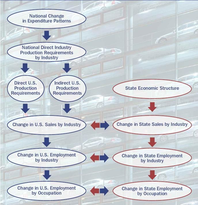
III. METHODOLOGY modeling system, these states impacts are consistent with
The economic and employment effects of enhanced impacts at the national level, an important fact that adds
CAFE standards were estimated using the MISI model, to the credibility of the results since there is no
data base, and information system. A simplified version “overstatement” of the impacts at the state level.
of the MISI model as applied here is summarized in
Figure 1. IV. ESTIMATES OF NATIONAL IMPACTS
The first step in the MISI model involves translation of A. Deriving the Estimates
increased expenditures for reconfigured motor vehicles Estimating the costs in 2030 of implementing the
meeting the revised CAFE standards into per unit output enhanced CAFE Standards is fairly straightforward.
requirements from every industry in the economy. 19 - Using data from the EPA/NHTSA/CARB Technical
Second, the direct output requirements of every industry Assessment Report and data provided by the Union of
affected as a result of the revised CAFE standards are Concerned Scientists, including sales of cars and light
estimated, and they reflect the production and technology trucks, and accounting for the per vehicle additional
requirements implied by the enhanced CAFE standards. costs, provides estimates of the additional costs in the
These direct requirements show, proportionately, how U.S. economy as a result of the new standards.20 As
much an industry must purchase from every other shown in Table 3, the additional per vehicle costs range
industry to produce one unit of output. Direct from about $850 (2009 dollars) light trucks and cars
requirements, however, give rise to subsequent rounds of under the 3% scenario and increase to nearly $3,200 for
indirect requirements. The sum of the direct plus the cars and light trucks under the 6% scenario. The
indirect requirements represents the total output resulting additional costs to consumers range from $26.7
125ISSN: 2277-3754
ISO 9001:2008 Certified
International Journal of Engineering and Innovative Technology (IJEIT)
Volume 4, Issue 7, January 2015
billion under the 3% scenario to $58.6 billion under the liquid fuel costs to the consumer will be higher. Taking
6% scenario. the Reference Case miles traveled and applying it to the
Table 3. LDV Market in 2030 under CAFE Scenarios estimated stock efficiency estimates from the 2011
Annual Energy Outlook (AEO 2011), total U.S. fuel
consumption levels can be estimated.21 Comparing the 3-
6% CAFE scenarios to the Reference Case results in
estimated stock fuel savings which range from 20 billion
gallons under the 3% scenario, to 39 billion gallons under
the 6% scenario -- Table 4. In order to estimate a value
of this savings to the U.S. economy, the AEO 2011
Reference Case price of $3.64 per gallon was used, and
adjusted to decrease incrementally to $3.54 in the 6%
case. This resulted in a range of estimates of fuel savings
Source: EPA/NHTSA/CARB Technical Assessment under the 3% and 6% scenarios of $78 billion to $152
Report and the Union of Concerned Scientists, Reference billion.
Case and 3% through 6% Side Cases; and MISI; 2012.
B. Estimated National Impacts in 2030
For the modeling effort, the CAFE scenarios and
respective costs (Table 3) were compared to the business
as usual (BAU) scenarios and their respective costs
(Table 4). Because in all CAFE scenario cases the
additional costs in the U.S, economy of the vehicles are
less than the additional costs of the fuel, residual
consumer expenditures were allocated to the Final
Demand category of Personal Consumption Expenditures.
This methodology ensures that the application is a net
analysis, comparing identical amounts spent by
consumers in 2030, but with a very different expenditure
pattern. Under the CAFE scenarios the consumer is
purchasing more expensive LDV’s outfitted with
advanced technology, and under the respective BAU
scenario the consumer is purchasing a higher level of
liquid fuel for the vehicle.
Table 4. LDV Fuel Expenditures in 2030 under CAFE
Scenarios
Source: U.S. Energy Information Administration,
Annual Energy Outlook 2011; EPA/NHTSA/CARB
Fig.1. Use of the MISI Model to Estimate the Economic Technical Assessment Report and the Union of
and Jobs Impacts of Increased CAFE Standards Concerned Scientists; Reference Case and 3% through
6% Side Cases; and MISI; 2012.
Source: Management Information Services, Inc., 2012. Across all economic categories, the impacts of the
CAFE 6%, 5%, 4%, and 3% scenarios higher economic
Estimating the costs of not implementing the CAFE and jobs impacts than the (BAU) case – Table 5. The net
Standards is not as straightforward. Without the new positive impacts of the 6% scenario on the U.S. economy
standards, LDV stock efficiency levels will stagnate and are estimated to be:
126ISSN: 2277-3754
ISO 9001:2008 Certified
International Journal of Engineering and Innovative Technology (IJEIT)
Volume 4, Issue 7, January 2015
Gross economic output (sales), $31.2 billion As shown in Figures 2 to 5, each of the four enhanced
higher CAFE scenarios results in substantial economic and jobs
Employment, 684,000 higher benefits to the U.S. economy in 2030. Further, the
Personal income, $20.5 billion higher greater the increase in required mpg, the larger are the
Local, State and Federal taxes, $18.8 billion benefits. For example:
higher Figure 2 shows that U.S. gross economic output
Table 5. Summary of 2030 National Impacts (sales) increases from more than $15 billion (2009
3% 4% 5% 6% dollars) under the 3% scenario to more than $31 billion
Scenario Scenario Scenario Scenario (2009 dollars) under the 6% scenario.
Gross $15.5 $21.3 $26.6 $31.2 Figure 3 shows that the U.S. jobs created
Economic increase from more than 350,000 under the 3% scenario
Output to nearly 700,000 under the 6% scenario.
(billions)
Figure 4 show that U.S. personal income
Jobs 352 484 603 684
(thousands) increases from more than $10 billion (2009 dollars) under
Personal $10.2 $14.2 $17.6 $20.5 the 3% scenario to more than $20 billion (2009 dollars)
Income under the 6% scenario.
(billions) Figure 5 shows that U.S. federal, state, and local
Tax $9.3 $12.7 $15.8 $18.8 government tax revenues increase from more than $9
Revenues billion (2009 dollars) under the 3% scenario to nearly $19
(billions) billion (2009 dollars) under the 6% scenario.
Source: Management Information Services, Inc., 2012.
$35
The net positive impacts of the 5% scenario on the U.S.
$30
economy are estimated to be:
Billion 2009 Dollars
Gross economic output (sales), $26.6 billion $25
higher
Employment, 603,000 higher $20
Personal income, $17.6 billion higher
Local, State and Federal taxes, $15.8 billion $15
higher
$10
The net positive impacts of the 4% scenario on the U.S.
economy are estimated to be: $5
Gross economic output (sales), $21.3 billion
higher $0
Employment, 484,000 higher 3% Scenario 4% Scenario 5% Scenario 6% Scenario
Personal income, $14.2 billion higher
Local, State and Federal taxes, $12.7 billion Fig.2.Impacts on U.S. Gross Economic Output (Sales) in
2030
higher
Source: Management Information Services, Inc., 2012.
The net positive impacts of the 3% scenario on the U.S.
economy are estimated to be:
Gross economic output (sales), $15.5 billion 700
higher
600
Employment, 352,000 higher
T housands of Jobs
Personal income, $10.2 billion higher 500
Local, State and Federal taxes, $9.3 billion
higher 400
The employment concept used is a full time equivalent 300
(FTE) job in the U.S. An FTE job is defined as 2,080
200
hours worked in a year’s time, and adjusts for part time
and seasonal employment and for labor turnover. Thus, 100
for example, two workers each working six months of the
year would be counted as one FTE job. An FTE job is 0
the standard job concept used in these types of analyses 3% Scenario 4% Scenario 5% Scenario 6% Scenario
and allows meaningful comparisons over time and across
jurisdictions. Fig 3. Impacts on U.S. Jobs in 2030
Source: Management Information Services, Inc., 2012.
127ISSN: 2277-3754
ISO 9001:2008 Certified
International Journal of Engineering and Innovative Technology (IJEIT)
Volume 4, Issue 7, January 2015
Table 6. Net Employment Impacts of 6% Scenario in
$25 Industries Most Affected (Thousands of FTE jobs)
Retail trade 77
$20 Hospitals and nursing and residential care facilities 72
Billion 2009 Dollars
Food services and drinking places 66
Motor vehicles, bodies and trailers, and parts 63
$15 Other services, except government 57
Ambulatory health care services 54
Construction 39
$10 Social assistance 26
Wholesale trade 25
$5 Educational services 24
-
Petroleum and coal products -2
$0 Water transportation -2
3% Scenario 4% Scenario 5% Scenario 6% Scenario Federal Reserve banks, credit intermediation, and related activities -3
Chemical products -3
Fig 4. Impacts on U.S. Personal Income in 2030 Pipeline transportation -4
Source: Management Information Services, Inc., 2012.
Computer systems design and related services -15
Management of companies and enterprises -16
20 Oil and gas extraction -24
18 Support activities for mining -26
Rental and leasing services and lessors of intangible assets -31
16
Billion 2009 Dollars
14 Net Total 684
12 Source: Management Information Services, Inc., 2012.
10 Table 7. Net Employment Impacts of 3% Scenario in
Industries Most Affected (thousands of FTE jobs)
8
Retail trade 43
6 Hospitals and nursing and residential care facilities 39
4 Food services and drinking places 35
2 Motor vehicles, bodies and trailers, and parts 31
Other services, except government 30
0
Ambulatory health care services 30
3% Scenario 4% Scenario 5% Scenario 6% Scenario
Construction 15
Fig 5. Impacts on U.S. Federal, State, and Local Social assistance 14
Government Tax Revenues in 2030 Educational services 13
Source: Management Information Services, Inc., 2012. Wholesale trade 13
-
C. Estimated Industry Impacts in 2030
We estimated the jobs impacts of the different Water transportation -1
scenarios in 70 NAICS industries. 22 While net Other transportation and support activities -1
employment in most industries increased under each Federal Reserve banks, credit intermediation, and related activities -1
scenario, net jobs were lost in some industries. As shown Chemical products -2
in Tables 6 and 7 and Figures 6 and 7, the jobs gained in Pipeline transportation -2
various industries greatly exceed the jobs lost in others. 23 Management of companies and enterprises -8
Some industries consistently gain jobs under each
Computer systems design and related services -8
scenario; these include Retail Trade, Hospitals and
Oil and gas extraction -12
Nursing Facilities, Motor Vehicles and Parts,
Construction, and Educational Services. Other industries Support activities for mining -14
consistently lose jobs under each scenario; these include Rental and leasing services and lessors of intangible assets -16
Rental and Leasing Services, Mining Support Activities,
Oil and Gas Extraction, Pipeline Transportation, and Net Total 352
Petroleum and Coal Products. Source: Management Information Services, Inc., 2012.
128ISSN: 2277-3754
ISO 9001:2008 Certified
International Journal of Engineering and Innovative Technology (IJEIT)
Volume 4, Issue 7, January 2015
V. ESTIMATES OF STATE IMPACTS B. Impacts on States’ GDP
A. Deriving State Level Impacts Tables 8 and 9 illustrate the net impact on each state
We estimated the pattern of regional distribution of the GDP of the 6% and the 3% enhanced CAFE scenarios: 24
national impacts. For this, state regional input-output Table 8 shows the state GDP impacts of the 6% scenario
location quotients were derived using comparable U.S. and Table 9 shows the state GDP impacts of the 3%
Bureau of Economic Analysis regional data for 2009 at scenario.
the 70-order industry level. The national economic gross Table 8: Net Impacts on State Gross Economic Output of
output impacts for the four scenarios were distributed by the 6% Scenario (Millions of 2009 dollars)
MISI’s version of the state- and industry-level GDP State GDP Impact
accounts database. The national employment impacts for Rank
Alabama 1,620 9
the four scenarios were distributed by MISI’s version of
Alaska -4,350 51
the state- and industry-level employment database. These Arizona 1,410 29
resulted in state-by-industry economic and employment Arkansas 180 42
impacts that were summed to derive state totals. California 5,230 40
80 Colorado -1,360 45
Connecticut 1,390 26
70 Delaware 190 39
District of Columbia 460 33
T housands of Jobs
60 Florida 4,200 28
50 Georgia 3,150 16
Hawaii 260 35
40 Idaho 420 17
Illinois 4,110 23
30
Indiana 4,610 2
20 Iowa 1,400 7
Kansas 480 36
10 Kentucky 2,290 3
0 Louisiana -8,490 49
Maine 340 21
3% Scenario 4% Scenario 5% Scenario 6% Scenario Maryland 1,510 30
Massachusetts 2,410 22
Retail Trade Motor Vehicles Construction Education Michigan 8,730 1
Fig 6. Net Job Gains in 2030 under the Scenarios: Minnesota 1,580 27
Selected Industries Mississippi 320 38
Source: Management Information Services, Inc., 2012. Missouri 2,160 11
Montana 0 43
Nebraska 740 13
0 Nevada 620 32
3% Scenario 4% Scenario 5% Scenario 6% Scenario New Hampshire 430 18
-10 New Jersey 1,980 34
New Mexico -1,430 46
-20 New York 7,370 20
T housands of Jobs
North Carolina 3,500 12
North Dakota -70 44
-30
Ohio 4,750 8
Oklahoma -4,360 48
-40 Oregon 1,550 10
Pennsylvania 3,390 25
-50 Rhode Island 320 19
South Carolina 1,950 4
-60 South Dakota 310 14
Tennessee 2,740 5
Texas -31,800 47
-70
Utah 420 37
Vermont 200 15
-80 Virginia 2,150 31
Rental & Leasing Mining Support Oil & Gas Pipelines Washington 2,070 24
West Virginia 110 41
Fig. 7. Net Job Losses in 2030 under the Scenarios: Wisconsin 2,520 6
Selected Industries Wyoming -2,530 50
Source: Management Information Services, Inc., 2012. Net Total 31,200
Source: Management Information Services, Inc., 2012
129ISSN: 2277-3754
ISO 9001:2008 Certified
International Journal of Engineering and Innovative Technology (IJEIT)
Volume 4, Issue 7, January 2015
Table 9: Net Impacts on State Gross Economic Output of 8 shows the states with the relatively largest GDP
the 3% Scenario (Millions of ’09 dollars) increases under the 6% Scenario and Figure 9 shows the
State GDP Impact states with the relatively largest GDP decreases Under the
Rank 6% Scenario.
Alabama 810 9
The rankings in these tables and figures are based on
Alaska -2,220 51
Arizona 710 29
the percentage impact of the state’s GDP. Under all of
Arkansas 90 41 the scenarios, GDP increases in 43 states and decreases in
California 2,650 40 only eight states.
Colorado -710 45 Figure 8 shows that the states whose GDP is increased
Connecticut 720 25 the most, on a percentage basis, from the 6% scenario
Delaware 100 38 (and generally the other scenarios as well) are Michigan
District of Columbia 230 33 and Indiana followed in descending order by Kentucky,
Florida 2,160 28 South Carolina, Tennessee, Wisconsin, Iowa, Ohio,
Georgia 1,600 16
Alabama, and Oregon. This is not surprising because
Hawaii 140 35
Idaho 210 17
these states are home to vehicle and vehicle parts
Illinois 2,070 23 manufacturing and related facilities.
Indiana 2,310 2 $9,000
Iowa 720 7
$8,000
Kansas 240 36
$7,000
Million 2009 Dollars
Kentucky 1,150 3
Louisiana -4,330 49 $6,000
Maine 170 19
Maryland 770 30 $5,000
Massachusetts 1,220 22 $4,000
Michigan 4,370 1
Minnesota 800 27 $3,000
Mississippi 160 39 $2,000
Missouri 1,100 11
$1,000
Montana 0 43
Nebraska 380 12 $0
Nevada 310 32
New Hampshire 220 18
New Jersey 1,020 34
New Mexico -730 46
New York 3,800 20
North Carolina 1,790 13
North Dakota -40 44 Fig 8. State GDP Increases Under the 6% Scenario (State
Ohio 2,390 8 Rankings Based on Percentage GDP Increases)
Oklahoma -2,230 48 Source: Management Information Services, Inc., 2012
Oregon 770 10
Pennsylvania 1,710 26
$0
Rhode Island 160 21
South Carolina 980 4
South Dakota 160 14 -$5,000
Tennessee 1,390 5
Million 2009 Dollars
Texas -16,300 47 -$10,000
Utah 200 37
Vermont 100 15
-$15,000
Virginia 1,080 31
Washington 1,050 24
West Virginia 50 42 -$20,000
Wisconsin 1,270 6
Wyoming -1,290 50 -$25,000
Net Total 15,500
Source: Management Information Services, Inc., 2012 -$30,000
The relative impacts on state GDPs of each of the -$35,000
scenarios are generally similar, and those states affected
the most, negatively and positively, are generally the Fig 9. State GDP Decreases Under the 6% Scenario (State
Rankings Based on Percentage GDP Decreases)
same under each scenario. Figures 8 and 9 illustrate the
Source: Management Information Services, Inc., 2012
relative impacts on state GDP of the 6% scenario: Figure
130ISSN: 2277-3754
ISO 9001:2008 Certified
International Journal of Engineering and Innovative Technology (IJEIT)
Volume 4, Issue 7, January 2015
Figure 9 shows that the eight states whose GDP is The oil and gas extraction industry is one of the most
decreased the most, on a percentage basis, from the 6% labor extensive industries, with large contributions to the
scenario (and generally the other scenarios as well) are economy, but with relatively few employees per dollar of
Alaska, Wyoming, and Louisiana, followed by that economic activity. This is seen clearly in the Texas
Oklahoma, Texas, New Mexico, Colorado, and North example. While the oil and gas extraction industry
Dakota. This is not surprising: Each of these eight states contributes over six percent to the state’s GDP, the
is a major oil producer and demand for oil will be industry accounts for only about two percent of total
reduced significantly by the enhanced CAFE standards. employment in the state. Therefore, one can expect to see
much larger changes in state GDP compared to
C. Impacts on Jobs in Each State employment. What we are seeing in Texas in our
Tables 10 and 11 show the net impacts on jobs in each scenarios is that while GDP is decreasing due to volatile
state of the 6% and the 3% enhanced CAFE scenarios 25: declines in the oil and gas extraction industry,
Table 10 shows the state job impacts of the 6% scenario employment is not decreasing as much and is actually
and Table 11 shows the state job impacts of the 3% being overwhelmed by the positive indirect employment
scenario. impacts caused by the overall growth in the motor
The rankings in these tables are based on the vehicles industry and the overall growth in the U.S.
percentage impact on state employment. The relative economy driven by the consumer surplus.
impacts on states’ jobs of each of the scenarios are Figure 10 shows that, based on percentage job
generally similar, and those states affected the most, increases, under the 6% scenario (as is also true for the
negatively and positively, are generally the same under other three scenarios) Indiana and Michigan benefit the
each scenario. Figures 10 and 11 illustrate the relative most from the enhanced CAFE standards. As a
impacts on states’ jobs of the 6% scenario: Figure 10 hypothetical example of the significance of the jobs
shows the states with the relatively largest job increases impacts, consider that the current unemployment rate in
under the 6% Scenario -- the rankings in this figure are Indiana is 8.2 percent and in Michigan is 10.3 percent.
based on the percentage impact on state employment, and The jobs created under the 6% scenario would reduce
Figure 11 shows the states with the largest total job unemployment in these states by nearly a full percentage
increases under the 6% Scenario. Figure 12 shows the point: The unemployment rate in Indiana would decrease
differing impacts on jobs in four states – Michigan, Ohio, from 8.2 percent to 7.4 percent and the unemployment
North Carolina, and Texas – of each of the four scenarios. rate in Michigan would decrease from 10.3 percent to 9.6
Comparison of these tables and graphs with the percent.
previous ones yields interesting results. One of the most Other states whose jobs markets would benefit the
salient findings is that while GDP declines in eight states most, in relative terms, include Alabama, Kentucky,
under each of the four scenarios, jobs increase in each Tennessee, Ohio, North Carolina, Vermont, New
state across all four scenarios – except in Wyoming. This Hampshire, Oregon, New York, and Missouri. Vermont
is due to the differences in labor productivity and job and New Hampshire gain relatively few jobs, but both
creation in the different industries and sectors that are states have small labor forces. Many of the large states
gaining jobs and those that are losing jobs. impacted the most currently have unemployment rates at
There is thus a disparity not only in size, but also in or well above the national average, and would welcome
direction between the two projections of impacts in some the additional job creation resulting from the enhanced
states. For example, the disparity is greatest in the CAFE scenarios – as would all states.
difference between the projected economic gross output Figure 11 also yields an interesting perspective. This
loss of almost $32 billion in Texas under the 6% scenario, figure shows the states that gain the most jobs in absolute
while at the same time Texas is projected to gain almost terms under the 6% scenario (these states also generally
28,000 jobs. Because ours is a net analysis, three general gain the most jobs under the other three scenarios). This
trends are occurring simultaneously and pulling the Texas ranking is, of course, dominated by the states with the
economy in different directions: largest labor forces, and it is instructive to compare these
There is a loss of gasoline sales and rankings with the percentage job rankings shown in
thus a decrease in the demand for oil Figure 10. In many cases, the states gaining the largest
There is a stimulus to the motor vehicle numbers of jobs rank relatively low in percentage job
industry as LDV’s become more expensive gains; for example:
There is a stimulus to the general California gains, by far, the largest
economy driven by the consumer savings as a net impact number of jobs (81,000), but in terms of percentage job
th
of the change in consumer purchases for those two gains ranks only 17
products Texas gains nearly 28,000 jobs, but
Because Texas accounts for well over half of U.S. ranks near the bottom at 47th in terms of percentage job
economic activity in the oil and gas extraction industry, it gains.
will be severely affected by the decreased demand for oil.
131ISSN: 2277-3754
ISO 9001:2008 Certified
International Journal of Engineering and Innovative Technology (IJEIT)
Volume 4, Issue 7, January 2015
Florida gains over 37,000 jobs, but than 32,000 jobs, Ohio gains nearly 34,000 jobs,
th
ranks 27 in terms of percentage job gains. California more than 81,000, and Indiana nearly 24,000
New Jersey gains 18,000 jobs, but jobs. However, job increases and decreases will be
th spread unevenly among different sectors and industries
ranks 34 in terms of percentage job gains.
Pennsylvania gains nearly 30,000 jobs, within each state, and there will thus be job shifts within
th states as well as among states.
but ranks 24 in terms of percentage job gains.
Table 10: Net State Job Impacts of the 6% Scenario
Conversely, some of the states with the highest (FTE jobs)
State Employment Impact
percentage job gains due to their relatively small labor
Rank
forces experience relatively small total job increases; for Alabama 13,600 3
example: Alaska 100 50
Arizona 11,000 38
Vermont gains only 1,800 jobs, but Arkansas 5,700 33
ranks 8th in terms of percentage job gains. California 81,000 17
New Hampshire gains only 3,600 jobs, Colorado 8,300 43
but ranks 9th in terms of percentage job gains. Connecticut 8,200 28
Delaware 2,100 29
Thus, in assessing the jobs impacts by state it is
District of Columbia 2,100 45
important to assess both the relative impact on the state’s
Florida 37,200 27
job market as well as the total number of jobs created in Georgia 21,100 23
each state. It is also important to realize that much of the Hawaii 3,000 37
total job growth will occur in states that rank relatively Idaho 3,400 21
low in terms of percent job growth. Illinois 31,100 19
Figure 12 shows the differing impacts on jobs in four Indiana 23,900 1
states – Michigan, Ohio, North Carolina, and Texas – Iowa 8,400 14
under each of the four scenarios. It illustrates that, while Kansas 6,800 31
there are some relative differences in job gains, states Kentucky 12,800 4
Louisiana 2,600 49
tend to benefit uniformly from the job creation under
Maine 3,200 20
each scenario. Maryland 11,900 35
It is also important to note here that these are net job Massachusetts 17,100 22
gains. Some jobs in certain sectors and industries will be Michigan 32,300 2
lost under each scenario. However, these job losses will Minnesota 14,500 18
be far exceeded by job gains in the states in other sectors Mississippi 5,300 36
and industries. Missouri 15,300 12
Nevertheless, the bottom line is that the enhanced Montana 1,900 40
CAFE standards analyzed here will have strongly positive Nebraska 5,000 25
Nevada 5,700 30
economic and job impacts, and several major conclusions
New Hampshire 3,600 9
emerge from this research. First, enhanced CAFE
New Jersey 18,000 34
standards would increase employment, although some New Mexico 2,300 46
industries and sectors will lose jobs: New York 48,100 11
Under the 3% scenario, net job creation North Carolina 25,500 7
in the U.S. will total 352,000, and every state except North Dakota 1,300 44
Wyoming will gain jobs. Ohio 33,900 6
Under the 4% scenario, net job creation Oklahoma 2,600 48
in the U.S. will total 484,000, and every state except Oregon 9,700 10
Pennsylvania 29,800 24
Wyoming will gain jobs.
Rhode Island 2,400 26
Under the 5% scenario, net job creation South Carolina 10,200 16
in the U.S. will total 603,000, and every state except South Dakota 2,300 13
Wyoming will gain jobs. Tennessee 17,900 5
Under the 6% scenario, net job creation Texas 27,800 47
in the U.S. will total 684,000, and every state except Utah 5,300 39
Wyoming will gain jobs. Vermont 1,800 8
Second, jobs in most industries and sectors increase, Virginia 15,600 41
Washington 14,300 32
but some industries and sectors would lose jobs, and even
West Virginia 2,600 42
in those that gain jobs, some workers may be displaced. Wisconsin 15,200 15
Third, there are also regional implications. Every state Wyoming -400 51
except Wyoming will gain substantial numbers of jobs -- Net Total 684,000
for example, under the 6% scenario Michigan gains more Source: Management Information Services, Inc., 2012.
132ISSN: 2277-3754
ISO 9001:2008 Certified
International Journal of Engineering and Innovative Technology (IJEIT)
Volume 4, Issue 7, January 2015
Table 11: Net State Job Impacts of the 3% Scenario
50,000
(FTE jobs)
State Employment Impact 40,000
Rank 30,000
Jobs
Alabama 6,900 3
Alaska 0 50 20,000
Arizona 5,700 38 10,000
Arkansas 2,900 33
California 41,700 18 0
Colorado 4,200 43
Connecticut 4,300 28
Delaware 1,100 27
District of Columbia 1,200 45
Florida 19,200 29
Georgia 10,800 25 Fig 10. State Job Increases Under the 6% Scenario (State
Hawaii 1,500 37 Rankings Based on Percentage Employment Increases)
Idaho 1,700 23 Source: Management Information Services, Inc., 2012.
Illinois 16,000 19
Indiana 12,100 1 90,000
Iowa 4,300 14 80,000
Kansas 3,500 31 70,000
Kentucky 6,500 4 60,000
Jobs
50,000
Louisiana 1,300 49 40,000
Maine 1,700 16 30,000
Maryland 6,100 36 20,000
Massachusetts 8,900 21 10,000
0
Michigan 16,400 2
Minnesota 7,500 17
Mississippi 2,800 35
Missouri 7,900 12
Montana 1,000 40
Nebraska 2,600 26
Fig 11. State Job Increases Under the 6% Scenario (State
Nevada 2,900 30
Rankings Based on Total Employment Increases)
New Hampshire 1,900 9 Source: Management Information Services, Inc., 2012.
New Jersey 9,400 34
New Mexico 1,200 46
New York 25,000 11 35,000
North Carolina 13,000 7
30,000
North Dakota 700 44
Ohio 17,300 6 25,000
Oklahoma 1,300 48
Jobs
20,000
Oregon 5,000 10
Pennsylvania 15,600 22 15,000
Rhode Island 1,300 24
South Carolina 5,200 20
10,000
South Dakota 1,200 13 5,000
Tennessee 9,100 5
Texas 14,300 47 0
Utah 2,700 39 3% 4% 5% 6%
Vermont 900 8 Scenario Scenario Scenario Scenario
Virginia 8,000 41
Washington 7,400 32
Michigan Ohio North Carolina Texas
West Virginia 1,400 42
Wisconsin 7,800 15 Fig 12. Job Impacts in Selected States across the Four
Wyoming -200 51 Scenarios
Net Total 352,000 Source: Management Information Services, Inc., 2012.
Source: Management Information Services, Inc., 2012.
133ISSN: 2277-3754
ISO 9001:2008 Certified
International Journal of Engineering and Innovative Technology (IJEIT)
Volume 4, Issue 7, January 2015
VI. FINDINGS AND CONCLUSIONS New Mexico, Colorado and North Dakota. However, all
From the research summarized here, we derive the these states, except Wyoming, would see net job gains as
following major findings and conclusions: money is shifted away from the oil industry to sectors of
Each of the four scenarios covering the the economy that deliver more jobs per dollar spent by
range of new standards assessed for CAFE mileage and consumers.
GHG emissions improvements -- annual emissions In sum, the research summarized here indicates that
reductions and fuel-economy improvements of three, enhanced CAFE standards would have strongly positive
four, five and six percent per year for the years 2017-25 -- economic and job benefits. Our findings indicate that
would yield substantial economic and job benefits for the increased CAFE standards will not harm the U.S.
U.S. economy in 2030. This includes net jobs gains in 49 economy or destroy jobs. Hopefully, the information
states. provided here can inform future policy debates over
The greater the improvements in fuel CAFE standards.
economy and GHG emissions, the greater the economic
benefits. For example, nearly 700,000 new jobs would be ACKNOWLEDGEMENT
created under the six percent scenario, compared to only The authors are grateful to Carol Lee Rawn, Angela
about 350,000 jobs under the three percent scenario. Bonarrigo, Peyton Fleming, Steve Tripoli, David
Domestic U.S. auto industry job Friedman, and Brad Markell for assistance in the course
creation would increase under all four scenarios, of this work, and to several anonymous referees for
including 63,000 new, full-time domestic auto jobs in comments on an earlier draft. This research was
2030 under the six percent scenario. supported by Ceres.
Stronger fuel economy and GHG
standards would produce broad economic benefits. These REFERENCES
include significant consumer savings at the pump, which [1] Baum, Alan and Daniel Luria, Driving Growth: How Clean
Cars and Climate Policy Can Create Jobs,” report prepared
would shift significant consumer spending away from the for the Natural Resources Defense Council, United Auto
oil industry and towards other parts of the economy, such Workers and Center for American Progress by The
as retail trade, food, and health care. Planning Edge and the Michigan Manufacturing
The six percent scenario would Technology Center, March 2010.
generate an estimated $152 billion in fuel savings in 2030 [2] Bezdek, Roger H., and Robert M. Wendling. “Potential
compared to business as usual. Of the $152 billion saved Long-term Impacts of Changes in U.S. Vehicle Fuel
at the pump, $59 billion would be expected to be spent in Efficiency Standards,” Energy Policy, Vol. 33, No. 3
the auto industry, as drivers purchase cleaner, more (February 2005), pp. 407-419.
efficient vehicles. The remaining $93 billion will be [3] Citi Investment Research, “Fuel Economy Focus,
spent across the rest of the economy, from retail Perspectives on 2020 Industry Implications,” March 2011.
purchases, to more trips to restaurants to increased [4] “CAFE to Cost 82,000 Jobs,” Motor Trend, July 1, 2008.
consumer spending on health care.
All of the scenarios would deliver net [5] Central Valley Chrysler-Jeep, Inc. v. Goldstene, 529 F.
Supp. 2d 1151 (E.D. Cal. 2007);
job gains in 49 states, with the biggest winners on a
percentage basis being Indiana, Michigan, Ohio, and New [6] “Energy Independence and Security Act of 2007,” Public
York. Other states that would see the most job growth on Law 110-140, December 19, 2007.
a percentage basis include Alabama, Kentucky, [7] Green Mountain Chrysler Plymouth Dodge Jeep v.
Tennessee, North Carolina, Vermont, New Hampshire, Crombie, 508 F.Supp.2d 295 (D. Vt. 2007).
Oregon and Missouri. In terms of the total number of [8] “Improving Energy Security, American Competitiveness
new jobs, California and New York would see the biggest and Job Creation, and Environmental Protection Through a
gains, and other winners would include Florida, Ohio, Transformation of Our Nation’s Fleet of Cars And
Michigan Illinois, Pennsylvania, Texas, North Carolina, Trucks,” Presidential Memorandum issued May 21, 2010,
Indiana, Georgia and New Jersey. Wyoming is the only published at 75 Fed. Reg. 29399 (May 26, 2010).
state that would lose jobs. [9] Management Information Services, Inc., More Jobs Per
Effects on national and state GDP Gallon: How Strong Fuel Economy/GHG Standards Will
would be overwhelmingly positive. States seeing the Fuel American Jobs, report prepared for Ceres,
Washington, D.C., August 2011.
biggest percentage GDP gains under the strongest fuel
efficiency standard have large auto industry sectors. The [10] Massachusetts v. Environmental Protection Agency, 549
biggest gainers would be Michigan and Indiana, followed U.S. 497 (2007).
by Kentucky, South Carolina, Tennessee, Wisconsin, [11] National Academy of Sciences, National Research
Iowa, Ohio, Alabama and Oregon. Some states would Council, Committee on the Assessment of Technologies
see net GDP decreases under this same scenario. These for Improving Light-Duty Vehicle Fuel Economy,
are primarily oil-producing states such as Alaska, Assessment of Technologies for Improving Light Duty
Wyoming and Louisiana, followed by Oklahoma, Texas,
134ISSN: 2277-3754
ISO 9001:2008 Certified
International Journal of Engineering and Innovative Technology (IJEIT)
Volume 4, Issue 7, January 2015
Vehicle Fuel Economy, Washington, D.C., National
Academies Press, 2011.
[12] National Academy of Sciences, National Research
Council, Real Prospects for Energy Efficiency in the
United States, Washington, D.C.: National Academies
Press, December 2009.
[13] National Academy of Sciences, National Research
Council, America’s Energy Future: Technology and
Transformation, Washington. D.C.: National Academies
Press, 2009.
[14] North American Industry Classification System,
www.census.gov/eos/www/naics.
[15] Office of Transportation and Air Quality, U.S.
Environmental Protection Agency, Office of International
Policy, Fuel Economy, and Consumer Programs, National
Highway Traffic Safety Administration, U.S. Department
of Transportation, and California Air Resources Board,
California Environmental Protection Agency, Interim Joint
Technical Assessment Report: Light-Duty Vehicle
Greenhouse Gas Emission Standards and Corporate
Average Fuel Economy Standards for Model Years 2017-
2025, September 2010.
[16] “President Obama Announces Historic 54.5 mpg Fuel
Efficiency Standard,” The White House, June 29, 2011.
[17] Union of Concerned Scientists, “2030 Impacts of Fuel
Efficiency and Global Warming Pollution Standards,” June
2011.
[18] U.S. Energy Information Administration, Annual Energy
Outlook 2011, 2011.
[19] U.S. Environmental Protection Agency, Inventory of U.S.
Greenhouse Gas Emissions and Sinks: 1990 – 2007, 2009;
[20] U.S. Environmental Protection Agency, Office of
Transportation and Air Quality, “Interim Joint Technical
Assessment: Light-Duty Vehicle Greenhouse Gas
Emission Standards and Corporate Average Fuel Economy
Standards for Model Years 2017-2025.” 2010.
135You can also read


