Fiscal Multipliers and Policy in a Model of Goods, Labor and Credit Market Frictions - N. Petrosky-Nadeau Etienne Wasmer May 2014, Mainz
←
→
Page content transcription
If your browser does not render page correctly, please read the page content below
Fiscal Multipliers and Policy in a Model of
Goods, Labor and Credit Market Frictions

     N. Petrosky-Nadeau    Etienne Wasmer

       Carnegie Mellon    Sciences Po, CEPR

                 May 2014, Mainz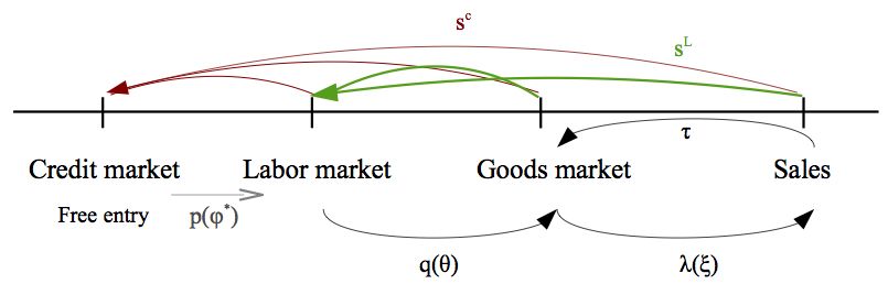
Introduction

    �   We develop our model of credit, goods and labor market
        frictions to study fiscal stimulus and fiscal multipliers
          �   Fiscal multiplier : GDP impact of an additional unit of
              public spendings (The New Palgrave, Chinn 2013)
          �   May be 1, 0, static, dynamic (lagged impact), long term
              (ratio of cumulated GDP impact over cumulated spendings)
    �   Renewed interest for these questions since the financial
        crisis
          �   State (as well as central bank interventions) have been
              massive in most Western economies.
Introduction
� Further, fiscal multipliers may vary :
� within cycles
� may be asymmetric (stimulus vs. consolidation impact)
� according to the position with respect to the “output gap”
or to the distance to some “steady-state”
� between cycles
� according to the nature of the recession ; e.g. financial
recessions
� according to its financing, origin of creditorsIntroduction
� Empirical litterature : Auerbach and Gorodnichenko (2012a
and b) have found that fiscal multipliers in the US may be
as large as 2.5 in a recession and close to zero in an
expansion; and in the same range in a panel of OECD
countries including France, Germany, Italy and Canada
� Convergent with several recent IMF reports or papers
(World Economic Outlook 2012, Batini et alii. 2012; Baum
et alii. 2012, Blanchard and Leigh 2013
� What are the existing theoretical ingredients?Introduction
� Two main mechanisms for multipliers greater than 1:
� Articulation with monetary policy : as the economy
approaches the zero lower bound on nominal interest rates,
central banks cannot prevent deflationary effects of fiscal
consolidation and therefore a fiscal stimulus avoids the
deflation trap
� Price and wage rigiditiesIntroduction
� On the first effect : Christiano, Eichenbaum, and Rebelo
(2011) found very large fiscal multipliers (more than 3) in a
DSGE setting, while Hall (2009) argue that multiplier may
be around 1.7 in a similar situation
� On the second: quite hard to obtain multipliers. Why?
Well explained by Woodford (2001)Introduction
� Think of a competitive economy first:
� output Yt as a function f of hours worked Ht
� consumed in equilibrium by households (Ct ) or government
(Gt )
� log linearizing f (Ht ) = Yt = Ct + Gt under the optimal
choice v � (Ht ) = u� (Ct ) where v(Ht ) is disutility for hours
worked and u(Ct ) is utility from consumption
� implies a fiscal multiplier dYt /dGt = ηu /(ηu + ηv )
� where ηu = −Cu”/u� ≥ 0
� and ηv is the elasticity of the disutility from supplying one
additional unit of output
� This multiplier is smaller than 1 : additional supply
requires additional effort (raises the implicit price of
consuming)Introduction
� The existence of a constant price markup m ≥ 1 does not
change the picture
� Only changes the equality of marginal utilities for leisure
and consumption : mv � (Ht ) = u� (Ct )
� hence without effect on the multiplier.
� To get round this smaller than 1 multiplier, varying
markups mt
� as put by Woodford, “the key to obtaining a larger multiplier
is an endogenous decline in the labor efficiency wedge”Neo-keynesian setup
� But not enough. Think of a simple monetary policy (simple
Taylor rule, nominal interest rate follows inflation and a
measure of GDP gap), leading to variations in nominal
interest rate
� If there is a monetary policy can set the real interest rate rt
to a constant
� a) away from a zero interest rate trap
� b) away from financial imperfections
� optimal intertemporal behaviour of households leads to
u� (Ct )
= e rt
βu� (Ct+1 )
� Under a constant real interest rate, constant consumption
with curved utility
� Hence, multipliers must be one: any additional public
spending is smoothed away in future consumptionPaleo-Keynesian instead?
� Keynes: general equilibrium interaction between markets.
Disequilibrium in a market (labor) lead to low demand and
thus higher unemployment
� Required a disequilibrium model with rationning and
agents sending signals to consume (e.g. Bénassy 1993)
� Same idea in matching models (Wasmer 2011) : aggregate
function of signals of agents in Bénassy is similar to Pissarides’s
rationalization (1990, chapter 1) of an aggregate matching
function: a technology that makes consistent the desired demand
and desired supply side of markets
� Here, we give a chance to the model to produce larger
multipliers, with frictions and matching in the goods
market, but also in the labor and credit markets (source of
amplification)Three symmetric frictions (C, L, G) and a timing
1. New project first requires liquidity: first match
2. Block creditor+project then requires labor : vacancies and
unemployment must match
3. The three agents form a new block which must finds
customers: matching between consumers and firms selling
� Agnostic: each matching block has a perfect market as a
limit case
� We have already quantified each of these blocks and
investigated the respective role of each frictions on dynamics
� All this is part of a broader research agenda of multiple
markets frictionsGoods markets
� Why search frictions in the goods market?
� Firm’s side:
� Advertising, 2% of GDP and procyclical (Hall 2012)
� Capacity utilization less than 100% (80%) so “vacant” firms
� In Bai et alii. words: “output is not equal to the
combination of inputs”
� Eg: restaurant food is sold if there are customers (does not
only depend on the number of tables)
� Consumers’ side:
� Time use surveys: shopping time is positive and procyclical
� Hence, consumption is also a function of transaction effort
(think of consumptions of services, or of the service of
durables goods)
� Evidence of product entry and exit (Broda and Weinstein
AER 10), turnover in product tastes
� Joint surplus and endogenous markupsEarlier paper (NPN-EW 2014): goods market frictions
fundamentally change the dynamics
1. Credit and goods market frictions are substitutable in generating
amplification of technology shocks
2. Goods market frictions are unique in generating persistence and
hump-shaped responses to shocks
3. Bridge the gap with data, both in terms of volatility (sd of logs) and
persistence (autocorr. in growth rates)
Table: Labor Market Second Moments
Standard deviation Autocorr. ∆θt Corr(U, V )
U V θ Lag 1 Lag 2
U.S. Data 0.13 0.14 0.27 0.68 0.36 -0.91
Baseline (CLG) 0.09 0.16 0.24 0.27 0.04 -0.79
Labor (L) 0.02 0.03 0.04 0.16 -0.04 -0.78
Credit-Labor (CL) 0.06 0.10 0.16 0.16 -0.05 -0.77
Goods-Labor (GL) 0.07 0.13 0.20 0.25 0.02 -0.80Role of goods market frictions vs. other frictions
Labor market tightness θ
0.18
Labor: L
0.16 Credit−Labor: CL
Goods−Labor: GL
0.14 Credit−Labor−Goods: CLG (Baseline)
Proportional change
0.12
0.1
0.08
0.06
0.04
0.02
0
0 5 10 15 20 25 30 35 40
Quarters
Figure: Comparing Frictions Impulse Responses to a Positive
Technology Shock.Mechanisms in the goods market
Explanation : mechanisms related to goods market frictions:
1. Expected surplus from production procyclical ; same for
expected surplus from exchange (consumption)
1.1 It follows that consumers’ search effort for goods:
procyclical ; eases matching in goods market, positive
feedback effect on firms
1.2 Bargained prices are countercylical but total revenue of the
firm still procyclical
2. Goods market tightness (ratio consumers to sellers):
countercylicalOverview of the model
� 3 types of agents: Banks, Investment projects
(entrepreneurs), Workers ; all three required to produce
�Only banks have access to storage and liquidity. Conversion
technology between numeraire and quasi-numeraire
� Lifecycle of a project: search for credit, then labor, then
consumers with endogenous transition rates
� Novelty in this paper:
� Concave utility, hence non-search goods are no longer a
numeraire but quasi-numeraire. 4 types of goods: search good
(1), a quasi-numeraire (0), a numeraire and leisure
� Matching frictions: Credit, Labor, Goods with two intensive
search margins
Market Matching Tightness Price Search effort
individuals firms
Credit ΩC (NC , BC ) φ ψ - -
Labor ΩL (V, U ) θ w - -
Goods ΩG (ēg,t ΞU,t , ēA,t NG,t ) ξ P eg eACredit, labor and goods market frictions
Four stages for the firm, subscript j
� j = c: search for credit, successful with probab p(φ)
� as in Wasmer and Weil (2004) and NPN-EW (AEJ Macro 2012),
ignored in the presentation, present in the calibration)
� Simply introduces an entry cost K(φ)
� j = v: vacancy searches for labor, successful with probab q(θ)
� j = g: search for consumer of the good, successful with probability
λ(ξ)
� j = π: profits, it ends with probability sC , sG ,sLSearch in the labor market
In subsequent stages (post credit) j = v, g, π, bank and project
continue to operate jointly as a firm of joint value
Jj,t = Ej,t + Bj,t
A number Vt of firms in stage v (vacancies) search for
unemployed workers U
Vt
� measure of market tightness : θt = Ut
ΩL (Vt ,Ut )
� labor market matching : Vt = q(θt ) with q � (θt ) < 0Matching on goods market
� Mass NG of firms ready to produce makes
advertising/selling effort eA to meets with a stock ΞU of
unmatched consumers who search for a product with
intensity eg
ΞU,t
� Concept for tightness in the goods market: ξt = NG,t
� Matching on goods market:
MG (ēg,t ΞU,t , ēA,t NG,t )
Firms: = λ(ξt , ēg,t , ēA,t ) ∂λ(ξt )/∂ξt > 0
NG,t
MG (ēg,t ΞU,t , ēA,t NG,t )
Consumers: = λ̌(ξt , ēg,t , ēA,t ) ∂ λ̌(ξt )/∂ξt < 0
ΞU,t
and λ̌(ξt ) = λt (ξt )/ξt .Consumption and income
� Two consumption goods: numeraire c0 and manufactured
c1 , with utility v(c1,t , c0,t )
� Second good c1 yields higher marginal utility but must be
found (frictions): manufacturing, some services
� First good: food exp. + utility
� Presumption: complementarity in consumption
� Search cost σ(eg ), with σ � (eg ) > 0 and σ �� (eg ) ≥ 0
� A short term budget constraint Pt c1,t + c0,t = Itd with
resources pooled across categories of workers (Merz (1995)
and Andofaltto (1996)):
Itd = (Πt + Nt wt + Gt − Tt )/Ξ̄ + ȳ 0
= [(Pt xt − Ω)Nπ,t − γVt − σA + Gt − Tt ] /Ξ̄ + ȳ 0
where ȳ 0 is self-production of a numeraire ; Gt and Tt are
fiscal transfers and taxesOverview of model with goods market frictions After hiring worker, firm must find a customer first to sell production Additional costs (worker must be paid even if there are no sales) and dynamics where transitions rates λ(ξ)
Overview of model - Single job creation equation

   Value of firm in recruiting stage equalizes cost and benefits and
   determines θt :
                          γ                1
                                       =       Et Jg,t+1
                        q(θt )
                        � �� �         � 1 + r��       �
               Cost of labor frictions Expected profits
Bellman equations
Bellman equations:
1
Jv,t = −γt + Et [qt Jg,t+1 + (1 − qt )Jv,t+1 ]
1+r
� � � �
1 − sL eA,t λt Jπ,t+1 eA,t λt sL Jv,t+1
Jg,t = −wt − σA,t + Et + (1 − )Jg,t+1 +
1+r ēA,t t
ēA,t 1+r
� L � � L �
1−s s Jv,t+1
Jπ,t = P t xt − w t − C Q + E t (1 − sG )Jπ,t+1 + sG Jg,t+1 +
1+r 1+r
� Small production cost CQ to ensure no production undertaken in
stage gDetermining price P
Consumer have utility v(c1,t , c0,t ) − σg (eg,t )
� � � �
1 eg,t λ̌t eg,t λ̌t
DU,t = v(0, c0,t ) − σ(eg,t ) + Et DM,t+1 + 1 − DU,t+1
1+r ēg,t ēg,t
1 − sL � G G
� sL
DM,t = v(c1,t , c0,t ) + Et s DU,t+1 + (1 − s )DM,t+1 + Et DU,t+1
1+r 1+r
� If we assume separability and with the short-run budget constraint :
v(c1,t , c0,t ) = b1 (xt ) + b0 (Itd − c1,t Pt )
� Denote by ∆v the difference operator across states (matched or
unmatched). Under linear utility for the numeraire, we have that
∆v = b1 (xt )
hence independent of both prices and disposable income : fiscal
multiplier here is 1: all in consumption of more numeraire
� We need concave utility to obtain a non-trivial multiplierDetermining price P
� Price bargaining is a natural solution: the total surplus to the
� �
consumption relationship is StG = (Jπ,t − Jg,t ) + DM,t − DU,t
� The good’s price is determined as
Pt = argmax (Jπ,t − Jg,t )1−αG (DM,t − DU,t )αG
, where αG ∈ (0, 1) is the share of the goods surplus going to the
consumer.
� Sharing rule is
�
(1 − αG ) (DM,t − DU,t ) = αG v0,t (Jπ,t − Jg,t )
� Hence time varying share of consumers: depends on their marginal
�
utility for quasi-numeraire v0,t :
�
αG v0,t
δ˜t = �
1 − αG + αG v0,t
�
� equal to αG with linear separable utility (v0,t = 1) ;
� �
� above αG if v0,t > 1, converges to 1 if v0,t → ∞ (starvation)
� �
� below αG if v0,t < 1, converges to 0 if v0,t = 0 (satiation of 0)Determining price P
� Price setting and choice of utility are key (of course): assume
v(c1,t , c0,t ) = b1 (c1,t ) + b0 (Itd − Pt c1t )
(+b01 ν0 (c0,t )ν1 (c1,t ))(not needed)
� Under linear separable utility: no impact of Itd , because price is
a weighted average of cost of producing and utility of consuming:
� �
Pt xt = αG [CQ − σA (1 − ησA )] + (1 − αG ) b1 (xt ) + σg (1 − ησg )
� Under non linear utility: there is an(noying) intertemporal term in
prices: same expression + future surpluses
� � � �
G G
ΛEt (1 − δ̃t )St+1 − ΛEt (1 − δ̃t+1 )St+1 (1)Determining price P
� A Kalai solution gets it simpler computionally: it reduces by one x
number of approx. terms in Chebyshev (here 3) the dimensionality of
the space state
� In the general case with decreasing marginal utility in quasi-numeraire
, prices react (positively) to Itd :
�
δ̃t [Pt xt − CQ + σA (1 − ησA )] = (1 − δ̃t ) b1 (xt ) + b0 (Itd − Pt xt ) − b0 (Itd ) + σg
� Higher income leads to more consumption of goods 0 in both
matched and unmatched states, thus to reduces the
quasi-numeraire utility gap from spending income into the search
good
� Same as complementarity between c0,t and c1,tOptimal search efforts
λ̌t
ēc,t σc� (e∗c,i,t ) = G
Et δ̃t+1 St+1 . (2)
1+r
� λt � �� �
ēA,t σA (eA,t ) = 1 − sL 1 − sC Et (1 − δ̃t+1 )St+1
G
(3)
1+r
� Since the marginal expected surplus is procyclical, so are the
search efforts of both sides of the goods market.
� Empirically confirmed by Hall (2013) for advertising efforts
� Further, combining the optimality conditions for the intensive
search margins with bargaining, we have:
ēA,t σA �
(eA,t ) Et (1 − δ̃t+1 )St+1
G � �� �
�
= ξ t × 1 − sL 1 − sC > 0
ēc,t σc (ec,t ) Et δ̃t+1 St+1
G
� Strategic complementarity arising from bilateral search effortIndeed! time use survey suggest procyclical search for
goods
Hours per day spent purchasing:
Goods and Services of which Consumer Goods of which Grocery shopping
2003 0.81 0.40 0.11
2004 0.83 0.41 0.10
2005 0.80 0.41 0.11
2006 0.81 0.40 0.10
2007 0.78 0.39 0.10
2008 0.77 0.38 0.10
2009 0.76 0.38 0.11
2010 0.75 0.37 0.10
2011 0.72 0.37 0.11
Source: http://www.bls.gov/tus/, Civilian Population, Table 1 and Table A1,Procyclical search for goods
TIme spent purchasing goods and service − ATUS 2003−2012
0.95 Aggregate
0.9 Employed
Unemployed
0.85 Not in Labor Force
Hours per day
0.8
0.75
0.7
0.65
0.6
0.55
0.5
2003 2004 2005 2006 2007 2008 2009 2010 2011 2012
BackWages
� For simplicity, we assume a wage rule that takes the
functional form
wt = χw (Pt xt )ηw , (4)
where ηw is the elasticity of wages to the marginal
production of labor in terms of the quasi-numeraire Pt xt
� Adapted from in Blanchard-Gali (2010), allows us to focus
on the role played by the elasticity of wages to prices for
fiscal multipliers
� Petrosky-Nadeau and Wasmer (2014) and Appendix explore
wage variants such as Nash-bargaining, one for which the
firm is in stage g, the other when the firm is in stage πLaws of motions
Consumers:
� � �� � � ��
ΞU,t+1 = (1 − λ̃t )ΞU,t + sC + 1 − sC sL + 1 − sL sG ΞM,t(5)
� �� �
ΞM,t+1 = 1 − sC 1 − sL (1 − sG )ΞM,t + λ̌t ΞU,t (6)
Firm:
� �� �� �
NG,t+1 = 1 − sC 1 − sL
(1 − λt )NG,t + sG Nπ,t + q(θt )Vt (7)
� �� �� �
Nπ,t+1 = 1 − sC 1 − sL (1 − sG )Nπ,t + λt NG,t . (8)
Workers
� � � �
U t+1 = sC + 1 − sC sL (1 − Ut ) + (1 − f (θt )) Ut (9)
1 − Ut = NG,t + Nπ,t = Nt+1 . (10)
Vacancies with imperfect markets: prior to vacancy creation, projects EC,t
and creditors (banks) BC,t must meet:
Vt+1 = p(φ)EC,t + [1 − q(θt )] Vt + sL Nt+1
= φp(φ)BC,t + [1 − q(θt )] Vt + sL Nt+1 . (11)Extension to credit markets
� The transition rates for investment projects and creditors
are given by:
ΩC (NC , BC )
= p(φ) with p� (φ) 0 (13)
BC
� Double free-entry of creditors and projects +
Nash-bargaining (share αC to the bank) leads to:
κB κI
Jv,t = Ev,t + Bc,t ≡ + =K
φ p(φ∗ )
∗ p(φ∗ )
κB 1 − α C
φ∗ = ∀t
κI α COverview of model - Single job creation equation
Value of firm in recruiting stage equalizes cost and benefits and
determines θt :
γ 1 − sc
+ = Et Jg,t+1
K(φ∗ )(1 + ot ) q(θ )
� �� � � �� t � � 1 + r�� �
Cost of credit frictions Cost of labor frictions Expected profitsIllustration with log linearization of the job creation
condition
Dynamics of job creation:
1 Sg
×
θ̂t = ηL Sg − K ×Et Ŝg,t+1
���� ���� � �� � � �� �
Elasticity : Labor frictions Credit frictions Goods frictions
� Financial multiplier from small firm surplus Sg − K(φ∗ )Equilibrium
The equilibrium is a set of policy and value functions for the consumers
{DM,t , DU,t , ēg,t } and firms {Jc,t , Jv,t , Jg,t , Jπ,t , ēA,t }; a set of prices rules in
goods, labor and credit; and stocks, measures of tightness in the markets
for goods, labor and credit {BC,t , NC,t , Vt , NG,t , Nπ,t , ΞU,t , ΞM,t , U t } and
{ξt , θt , φ}, overall 22 variables, such that 22 equations are satisfied:
1. Consumers’ value follows functions, with the search-effort optimality
conditions for consumers
2. Firm’s value functions in the vacancy stage, in the consumer stage and
in the profit stage, together with the optimal advertisment condition
3. Three definitions of credit, labor and goods market tightness as a
ratio of the searching stocks
4. A credit block with free-entry in the credit market for both projects
and banks (2 equations)
5. Prices in the goods, labor and credit markets are determined by Nash
bargaining given by conditions
6. Stock in the goods and labor markets follow seven law of motions, a
fixed total number of consumers, finally two identities between the
number of firms and the number of employed workers on the one
hand, and between the number of matched firms and the number of
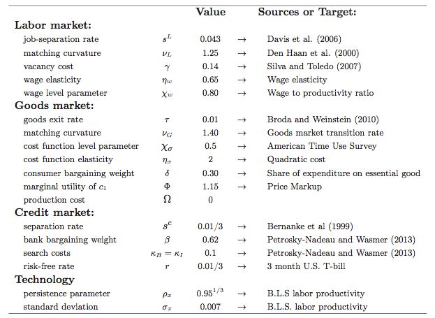
matched consumers on the other handCalibration: same as dynamic CLG model NPN-EW
(2004)
� Risk free rate r = 0.04 yearly
� Productivity: log xt = ρx log xt−1 + εxt ,
ρx = 0.983, σx = 0.0072
� Wage rule: bargaining or alternatively some recent macro
shortcut wt = χw (Pt xt )ηw NB Wage
� Den Haan et alii. (2012):
X1 X2
Mj (X1 , X2 ) = ν ν 1/νC , j = C, L, G
(X1 C +X2 C )Calibration: labor and credit markets
� Labor targets:
� 5.8% unemployment rate, job separation sc + (1 − sc )sL = 0.043
(Davis et alii. 2006), implies f
� Elasticity of wages to productivity ≈ 0.75,
� W/P =0.75
� Credit market target:
Bπ ρ−Bg w−Bl γ−Bc κ
� credit market’s share of GDP Σ = Y
= 2.5%Calibration: goods markets
� Price mark-up over cost of 15%
� Broda and Weistein (2010):
� average rate of product entry λ̃ = 0.22
� average product exit rate implies τ =0.01
� Cost of time searching in the goods market corresponds to
approximately 7% of wage income Time Use
� Φ : obtained from the target on the share of expenditures on primary
goods (food consumed at home plus utilities): 15%Calibration (monthly)
Government and debt
    �   Fiscal policies with some persistance known to economic
        agents and denote by ρG the first order auto-correlation of
        the policy
    �   For a given impulse policy Gt0 at time t0 , we denote by
          t0 (T ) the cumulated spending at horizon t, and
        Gcum
                                  t
                                  �               t
                                                  �
                      Gcum
                       t0 (t) =         Gt0+k =           ρkG Gt0
                                  k=0               k=0
                                  �∞
                                                      Gt 0
                     Gcum
                      t0 (∞) =          ρkG Gt0 =
                                                    1 − ρG
                                  k=0
    �   Debt repaid at a fixed interest rate rG , and is fully repaid
        in the long-run - quite at a slow pace though
    �   Short-run (T = 0) and the longer-run multipliers:
                                    �T
                                          ∆cum Yt0 +k
                         MG (T ) = k=0 �T
                                         k=0 Gt0+k
Exercise: fiscal stimulus (blue) or consolidation (red)
0.05
0.04
0.03
0.02
Net Transfer τ
0.01
0
−0.01
−0.02
−0.03
−0.04
−0.05
0 5 10 15 20 25 30
PeriodsStimulus: debt increases then decreases slowly
0.15
0.1
Government Debt
0.05
0
−0.05
−0.1
−0.15
−0.2
0 5 10 15 20 25 30GDP reacts quite fast
0.08
0.06
0.04
0.02
GDP
0
−0.02
−0.04
−0.06
−0.08
0 5 10 15 20 25 30
PeriodsFiscal shock affect forward value of goods surplus
0.04
Expected Goods mkt surplus 0.03
0.02
0.01
0
−0.01
−0.02
−0.03
−0.04
0 5 10 15 20 25 30
PeriodsFirms advertise more (or less in consolidation)
0.01
0.008
0.006
Firm Advertising
0.004
0.002
0
−0.002
−0.004
−0.006
−0.008
−0.01
0 5 10 15 20 25 30
PeriodsSame for consumer search effort
0.01
Consumer search effort 0.008
0.006
0.004
0.002
0
−0.002
−0.004
−0.006
−0.008
−0.01
0 5 10 15 20 25 30
PeriodsSome procyclicality of wages
0.03
0.02
0.01
Price P
0
−0.01
−0.02
−0.03
0 5 10 15 20 25 30
PeriodsEmployment reacts more slowly - persistence
−4
x 10
4
3
2
1
N pi
0
−1
−2
−3
−4
0 5 10 15 20 25 30
PeriodsFiscal multiplier quite high: 1.4
1.5
Expansionary policy
Contractionnary policy
1
Fiscal Multiplier (GDP)
0.5
0
−0.5
−1
−1.5
0 5 10 15 20 25 30
Time Horizon − MonthsSummary: compare a productivity shock and a fiscal
stimulus
� Sequence:
1. Positive fiscal stimulus ⇒ consumers consume more the
quasi-numeraire, whether matched or unmatched
2. At a constant price, more total surplus from consumption of
the search good because of decreasing marginal utility
(sacrifice of buying search goods is lower after the fiscal
expansion
3. Hence higher price, more firms advertising, more effort to
enter the market
4. Consumers meet search goods more frequently
4.1 Hence increase in consumer search effort
5. Amplification, hump-shape and the shock is more persistent.Technological shock: the same except for prices
Labr market tightness θ Expected value of worker E Sg
t t+1
20 1
% deviation
15
10 0.5
5
0 0
0 10 20 30 40 0 10 20 30 40
Expected firms goods matching rate Etλt+1 Expected Price Et Pt+2
0 0
% deviation
−1
−0.5
−2
−1
−3
−4 −1.5
0 10 20 30 40 0 10 20 30 40
Search effort Goods market tightness
1.5 0
% deviation
1 −2
0.5 −4
0 −6
0 10 20 30 40 0 10 20 30 40
Quarters Quarters
Figure: Propagation of a Positive Technology ShockSummary: compare a productivity shock and a fiscal
stimulus
� Sequence for a positive fiscal stimulus
1. Positive surplus shock ⇒ more firms enter
2. More competition to sell goods (both goods market
tightness and price decline)
3. Overall effect still positive for firms, BUT in addition...
4. .. consumers get higher income (only after the two
matching lags) and also meet search goods more frequently
4.1 Hence strong increase in consumer search effort
5. Amplification, hump-shape and the shock is more persistent.Sensitivity: specification of goods market frictions
We explore three additional variants.
1. Baseline: search effort by consumers
λ̃t /ēc,t
σ � (e∗c,i,t ) = Et [(D1,t+1 − D0,t+1 )]
1+r
2. Firm’s advertising effort
� λt /ēA,t � �
σA (e∗A,t ) = Et [Sπ,t+1 − Sg,t+1 ] 1 − sL (1 − sc )
1+r
3. Two sided effort : leads to a strategic complementarity
� (e � �
ēA,t σA A,t ) 1−δ � �
�
= 1 − sL (1 − sc ) ξt
ēc,t σc (ec,t ) δ
� �2
ēA,t
e.g. = if quadratic costs
ēc,t
4. Constant consumer effortSensitivity: specification of goods market frictions
Table: Labor market second moments: Extensions
Standard deviation Autocorr. ∆θt Corr(U, V )
U V θ Lag 1 Lag 2
U.S. Data 0.13 0.14 0.27 0.68 0.36 -0.91
Variant 1. Baseline 0.09 0.16 0.24 0.27 0.04 -0.79
Variant 2. Firm effort 0.08 0.24 0.28 0.16 -0.05 -0.77
Variant 3. Two sided effort 0.11 0.22 0.27 0.23 0.02 -0.79
Variant 4. Constant ec 0.07 0.21 0.23 0.17 0.01 -0.81Sensitivity: specification of wages
Table: Business Cycle Moments - Sensitivity to the Specification of
Wages
Baseline wage setting Nash bargained
ζw,p = 0.85 (instead of 0.75) wages
LMG frictions L frictions LMG frictions L frictions
a b a b a b a b
Vacancies 10.51 0.98 1.05 0.94 8.28 0.97 3.09 0.88
Unemployment 4.66 -0.44 0.44 -0.69 4.94 -0.47 0.16 -0.67
Labor tightness 13.74 0.90 1.29 0.99 11.39 0.91 3.20 0.88
Wage 0.95 0.93 0.74 0.00 0.75 0.9 0.40 0.88
Consumption 0.99 0.99 1.00 0.00 0.95 0.9 0.66 0.75
Notes: H.-P. filtered (a) sd relative to GDP; (b) contemp. correlation
with GDP.Sensitivity: other parameters
� Wage Elasticity
Labor market tightness θ
10
Baseline response
9 Increased wage elasticity − ζw,p=0.75
% deviation from steady state
8
7
6
5
4
3
2
0 5 10 15 20 25
Quarters
� Good market matching function, elasticity
Labor market tightness θ
10
9 Baseline response
Increased Matching Elasticity − η =0.5
% deviation from steady state
G
8
7
6
5
4
3
2
0 5 10 15 20 25
QuartersSensitivity: other parameters
� Consumer search cost elasticity
Labor market tightness θ
11
Baseline response
10 Increased Search Cost Elasticity
Lower Search Cost Elasticity
% deviation from steady state
9
8
7
6
5
4
3
2
0 5 10 15 20 25
QuartersConclusion
1. Credit and goods market imperfections amplify the
response of labor market tightness to productivity
2. Only goods market imperfections provide persistence
3. Results robust to changes in goods market specification.Conclusion
This work: we have a simple framework to deal with aggregate
fiscal stimulus or consolidation
� Fiscal multipliers requires a concave utility
� Real effects you expect: increases in output and
employment ; but you can quantify them.
� E.g. : are fiscal multipliers countercyclical? Next talk when
simulations will be readyBargained Wage
The wage rule in this case is
�
argmax (Sg,t − Sl,t )1−α (Wg,t − Ut )α in stage g
wt =
argmax (Sπ,t − Sl,t )1−α (Wπ,t − Ut )α in stage π,
where Wg and Wπ are the asset values of employment to a
worker, and U is the value of unemployment. The resulting
wage rules are
� � � �
r+sc L 1−sc K in stage g
αθ t γ + 1+r K − α 1 + s 1+r
+(1 − α)b
wt = � � � �
L 1−sc K
α P x − Ω − 1 + s in stage π.
t
�
t
� 1+r
c
+αθt γ + r+s K + (1 − α)b
1+r
BackSearch for goods
Average hours per day men and women
spent in various activities
Average h
A hours
per day
5.0
Men Women
4.0
30
3.0
2.2
2.0
1.3
1.0 0.6 0.6
0.3 0.4
0.0
Household activities Caring for and helping Purchasing goods and
household members services
NOTE: Data include all noninstitutionalized persons age 15 and over. Data include all days of the week and
are annual averages for 2008. Travel related to these activities is not included in these estimates.
SOURCE: Bureau of Labor Statistics
BackModel Equations
� � �
1 ei,t λ̃t ei,t λ̃t
D0,t = U (0, c0,t ) − σ(ei,t ) + Et D1,t+1 + 1 − D0
1+r ēt ēt
� �
1 − sc � �
D1,t = U (c1,t , c0,t ) + Et 1 − sL [τ D0,t+1 + (1 − τ )D1,t+1 ]
1+r
s + (1 − s ) sL
c c
+ Et D0,t+1 .
1+r
κB κI
Sc,t = 0 ⇔ + = Sl,t
p̂t pt
1 − sc
Sl,t = −γ + Et [qt Sg,t+1 + (1 − qt )Sl,t+1 ]
1+r
1 − sc �� �
Sg,t = −wt + Et 1 − sL [λt Sπ,t+1 + (1 − λt )Sg,t+1 ] + sL Sl,t+
1+r
1 − sc �� �
Sπ,t = Pt xt − w t − Ω + Et 1 − sL [(1 − τ )Sπ,t+1 + τ Sg,t+1 ] +
1+rModel Equations
λ̃t
ēt σ � (e∗it ) = Et [(D1,t+1 − D0,t+1 )] . (20)
1+r
(1 − δ) (D1,t − D0,t ) = δ (Sπ,t − Sg,t ) , (21)
(1 − β)Bl,t = βJl,t , (22)
� � � �
αθt γ + r+sc K − α 1 + sL 1−sc K + (1 − α)b
� 1+r � � 1+r
� � �
wt =
α Pt xt − Ω − 1 + sL 1−sc K + αθt γ + r+sc K + (1 − α
1+r 1+rModel Equations
� � � � ��
C0,t+1 = (1 − λ̃t )C0,t + sc + (1 − sc ) sL + 1 − sL τ C(24)
1,t
c
� L
�
C1,t+1 = (1 − s ) 1 − s (1 − τ )C1,t + λ̃t C0,t (25)
� �
Ng,t+1 = (1 − sc ) 1 − sL [(1 − λt )Ng,t + τ Nπ,t ] + q(θt )N(26)
l,t
c
� L
�
Nπ,t+1 = (1 − s ) 1 − s [(1 − τ )Nπ,t + λt Ng,t ] . (27)
� �
ut+1 = sc + (1 − sc ) sL (1 − ut ) + (1 − f (θt )) ut (28)
1 − ut = Ng,t + Nπ,t . (29)Broda-Weinstein
� Broda and Weinstein (2010) carefully documented the
magnitude of flows of entry and exit of goods in a typical
household’s consumption basket.
� Unique data set of 700 000 products with bar codes purchased by
55 000 households (40% of all expenditures on goods in the CPI).
� They find large flows of entries and exits of "products” in a
typical consumer’s consumption basket, actually four times more
than is found in labor markets, and that a large share of product
turnover happens within firms.
� Over their 9 year sample period, 1994–2003, the product entry
rate, defined as the number of new product codes divided by the
stock, is 0.78 quarterly. The product exit rate, defined as the
number of disappearing product codes over the stock, is 0.72,
and 0.24 when weighted by expenditure share.
� Further, net product creation is strongly procyclical and
primarily driven by creation rather than destruction, which is
weakly countercyclical.Credit market frictions
Search on credit markets:
� Creditors (BC ) and investment projects (Nc ) meet to form
a firm
� Search costs: creditors κB ; investment projects κI
Nc,t
� Measure of credit market tighness: φt = Bc,t
Matching on credit markets:
MC (Bc,t , Nc,t )
= p(φt ) with p� (φt ) < 0.
Nc,tSearch on credit markets
Value of search on credit markets with free entry:
Ec,t = −κI + p(φt )El,t =0 (free-entry)
Bc,t = −κB + φt p(φt )Bl,t =0 (free-entry)
With Nash bargaining, (1 − β)Bl,t = βEl,t , implies
κB 1 − β
φ∗ = ∀t
κI β
Total transaction costs in stage c summarized as
κI κB
K(φ∗ ) ≡ + ∗
p(φ ) φ p(φ∗ )
∗You can also read