FPGA-Based Hardware Matrix Inversion Architecture Using Hybrid Piecewise Polynomial Approximation Systolic Cells - MDPI
←
→
Page content transcription
If your browser does not render page correctly, please read the page content below
electronics
Article
FPGA-Based Hardware Matrix Inversion Architecture
Using Hybrid Piecewise Polynomial Approximation
Systolic Cells
Javier Vázquez-Castillo 1 , Alejandro Castillo-Atoche 2           , Roberto Carrasco-Alvarez 3, *,
Omar Longoria-Gandara 4 and Jaime Ortegón-Aguilar 1
 1    Department of Engineering, University of Quintana Roo, Chetumal 77019, Mexico;
      jvazquez@uqroo.edu.mx (J.V.-C.); jortegon@uqroo.edu.mx (J.O.-A.)
 2    Department of Mechatronics, Autonomous University of Yucatán, Mérida 97203, Mexico;
      acastill@correo.uady.mx
 3    Department of Electronics, University of Guadalajara, Guadalajara 44430, Mexico
 4    Department of Electronics, Systems and IT, Western Institute of Technology and Higher Education,
      Tlaquepaque 45604, Mexico; olongoria@iteso.mx
 *    Correspondence: r.carrasco@academicos.udg.mx

 Received: 2 September 2019; Accepted: 20 November 2019; Published: 18 January 2020

 Abstract: The hardware of the matrix inversion architecture using QR decomposition with Givens
 Rotations (GR) and a back substitution (BS) block is required for many signal processing algorithms.
 However, the hardware of the GR algorithm requires the implementation of complex operations,
 such as the reciprocal square root (RSR), which is typically implemented using LookUp Table
 (LUT) and COordinate Rotation DIgital Computer (CORDICs), among others, conveying to either
 high-area consumption or low throughput. This paper introduces an Field-Programmable Gate Array
 (FPGA)-based full matrix inversion architecture using hybrid piecewise polynomial approximation
 systolic cells. In the design, a hybrid segmentation technique was incorporated for the implementation
 of piecewise polynomial systolic cells. This hybrid approach is composed by an external and
 internal segmentation, where the first is nonuniform and the second is uniform, fitting the curve
 shape of the complex functions achieving a better signal-quantization-to noise-ratio; furthermore,
 it improves the time performance and area resources. Experimental results reveal a well-balanced
 improvement in the design achieving high throughput and, hence, less resource utilization in
 comparison to state-of-the-art FPGA-based architectures. In our study, the proposed design achieves
 7.51 Mega-Matrices per second for performing 4 × 4 matrix operations with a latency of 12 clock
 cycles; meanwhile, the hardware design requires only 1474 slice registers, 1458 LUTs in an FPGA
 Virtex-5 XC5VLX220T, and 1474 slice registers and 1378 LUTs when a FPGA Virtex-6 XC6VLX240T
 is used.

 Keywords: field programmable gate arrays; matrix inversion; piecewise polynomial approximation;
 QR decomposition; systolic arrays

1. Introduction
     Matrix inversion is one of the most useful operations used in many signal processing algorithms
(SPA), where the efficient computation and accuracy of this operation are required. Important
areas such as image recovery, phased-array radar and sonar, wireless communication, control
applications, and others [1] require the efficient computations of the matrix inversion in real
time, specifically in Hardware (HW) implementations of wireless communication for designing
multiple-input multiple-output (MIMO) systems [2,3], in multiplicative noise generators using

Electronics 2020, 9, 182; doi:10.3390/electronics9010182                     www.mdpi.com/journal/electronics
Electronics 2020, 9, 182 2 of 14
autoregressive modeling [4], and more generally in the implementation of generic linear algebra
architectures [5].
Givens rotation (GR) is considered in this paper for implementing the QR decomposition (QRD)
due to its stability and accuracy [6,7], and at the same time, the GR technique allows a rapid prototyping
implementation on a parallel and pipelined systolic array structure. However, the HW design of the
standard GR requires the implementation of complex operations, such as square root (SR) and its
reciprocal (reciprocal square root (RSR)). In this sense, recent studies reported in References [8–11]
have been tackling this issue, incorporating lookup tables (LUT) and CORDIC (coordinate rotation
digital computer [12]) in order to compute the SR and RSR of the GR structure.
LUT-based designs are easy to implement, but the increase in memory is directly proportional
to the accuracy required by the HW architecture. The memory size could increase, even to
several megabytes, depending on the unit last place (ulp) value or according to a specific
signal-to-quantization-noise ratio (SQNR). On the other hand, CORDIC implementations have proved
its efficiency for computing complex operations such as SR, RSR, number division, sine, and cosine,
among others [12]. However, the accuracy of CORDIC implementation depends on the number of
algorithm’s iterations [13].
Specific fixed-point implementations of SR and RSR have been presented in References [14,15]
and can be used to improve the performance of the QRD hardware. However, such proposals are
based on iterative algorithms using several clock cycles for converging to the final result and require
significant HW resources as was discussed in References [16,17].
In this paper, a full matrix inversion architecture is designed. In the FPGA design, a hybrid
segmentation method is incorporated for the implementation of complex arithmetic functions in
combination with systolic and piecewise polynomial approximation (PPA) techniques. The resulting
hybrid PPA-systolic cells are integrated in the QRD and back-substitution modules. The developed
architecture demonstrates a better signal-quantization-to-noise ratio (SQNR), less execution time, and
a reduction in the area resources in comparison with state-of-the-art hardware architectures.
Although, recent publications of matrix inversion architectures and complex arithmetic operations
are in the current state-of-the-art literature, many of these works have been focused in the design of
LUT, CORDICs, or iterative techniques [18–20]. Other approaches have considered parallel hardware
implementations. For example, a parallel structure with inter-vector connectivity was implemented
in Reference [21], with an improvement in the time performance; however, the design is high
in the amount of area resources. Other studies, such as References [19,22], have focused on the
implementation with piecewise polynomial approximations or systolic arrays, but in these studies, the
designs present contributions only in time or area performance.
The rest of the paper is organized as follows: Section 2 reviews the background of matrix inversion
by QR decomposition using Givens rotations. Section 3 presents a parallel matrix inversion architecture
using hybrid piecewise polynomial approximation systolic cells. Section 4 analyzes the implementation
results and, then, compares the hardware performance with the state-of-the-art designs on FPGAs.
Section 5 presents a performance analysis discussion. Finally, Section 6 presents the concluding remarks.
2. Matrix Inversion by QR Decomposition
The matrix inverse procedure is based on QRD and back-subtitution, which are introduced in the
following subsections.
2.1. QRD Procedure
Let us consider a matrix A ∈ < m×n for m ≥ n; hence, the QRD can be expressed as A = QR,
where Q is an m × m orthogonal matrix, such that QQT = I (I is the identity matrix) and R is the
m × n upper triangular matrix. A technique for computing the matrix Q and R is by means of GR,
which has a computational complexity of O(3n2 (m − n/3)).Electronics 2020, 9, 182 3 of 14
The QRD consists of finding a matrix R and, subsequently, of pre-multiplying the matrix A by
several GR matrices, which are defined as G(i, j, θ ), where the entries (i, i ) and ( j, j) of matrix G are
equal to c = cos(θ ), the entry (i, j) is equal to s = sin(θ ), and the entry ( j, i ) is equal to −s. It is
important to note that the parameters (i, j) are fixed according to the corresponding rows of matrix A
for being rotated. On the other hand, θ is the degrees to be rotated. Therefore, the QRD procedure
consists of finding the GR matrices G1 , G2 , · · · , Gi such as G1 T × G2 T , · · · , Gi T A is a triangular upper
matrix. Since the GR matrices are orthogonal, the multiplication of multiple Givens matrices is also
orthogonal; hence, G1 T × G2 T , · · · , Gi T A = QT A = R.
In order to carry out the QRD hardware implementation, consider the following nomenclature:
Ri,j is the element allocated in row i and column j of matrix R and R(α1 : α2 , β 1 : β 2 ) is a sub-matrix of
R that contains all the elements corresponding to the rows from α1 to α2 and the columns from β 1 to
β 2 , respectively. Matrix Gr is defined as follows:
" # " #
cos(θ ) sin(θ ) c s
Gr = = , (1)
− sin(θ ) cos(θ ) −s c
where c2 + s2 = 1, and thus, the QRD can be implemented following Algorithm 1 as presented in
p. 252 in Reference [23].
Algorithm 1 QRD algorithm.
1: Parameter initialization: R = A
2: Begin of the QRD algorithm
3: for loop j = 1 : 1 : n − 1 do
4: for loop i = m : −1 : j + 1 do
5: To compute:
q
6: r = R2i−1,j + R2i,j
Ri−1,j Ri,j
7: Gr for c = r and s = − r
8: R(i − 1 : i, j : n) = GTr R(i − 1 : i, j : n)
2.2. Back-Substitution and Matrix Inverse Procedures
Once the matrix R is computed using Algorithm 1, it is necessary to calculate R−1 via the
back-substitution algorithm as RR−1 = I, where each of the matrices can be represented as follows:
r1,1 r1,2 · · · r1,m rinv1,1 rinv1,2 ··· rinv1,m
0 r2,2 · · · r2,m 0 rinv2,2 ··· rinv2,m
.. .. .. .. .. .. .. ..
. . . . . . . .
0 0 ... r
m,m 0 0 ... rinvm,m
(2)
1 0 ··· 0
0 1 ··· 0
= . .
. . .. .. .
. . . .
0 0 ··· 1Electronics 2020, 9, 182 4 of 14
Thus, using Equation (2), it is possible to write a system of linear equations as follows:
rm,m · rinvm,m = 1
rm−1,m−1 · rinvm−1,m + rm−1,m · rinvm,m = 0
.. (3)
.
r1,1 · rinv1,m + r1,2 · rinv2,m + . . . + r1,m · rinvm,m = 0
As can be seen, the first element of Equation (3) is computed directly as follows:
r j,j · rinv j,j = 1; 1 ≤ j ≤ m,
(4)
rinv j,j = r1 ,
jj
Also, substituting the value of rinv j,j in the second row of Equation (3) obtains rinvm−1,m . This
procedure is repeated until the entire system is solved in a back substitution fashion. Hence, once the
inverse matrix R−1 is obtained, it is possible to compute A−1 = R−1 QT = R−1 (R−1 )T AT .
Having analyzed the QRD Algorithm 1, it can be observed that the RSR operation is a crucial
part of the computations of this algorithm. In this sense, a hybrid PPA technique is presented in
the following subsection, which permits to improve the accuracy of the proposed hardware matrix
inversion architecture.
2.3. Evaluation of RSR Using Hybrid PPA Technique
The PPA technique is efficiently applied to evaluate the RSR function. Compared with uniformly
sized segments, the inclusion of a hybrid segmentation technique (conformed by an external and
internal segmentation, where the first is nonuniform and the second is uniform) is capable of reducing
the number of segments which significantly reduces the hardware resources [24].
It is remarked that this paper employs a hybrid segmentation, which is composed via the combination
of the uniform and nonuniform segmentation techniques. First, the RSR function is divided by using
a nonuniform segmentation technique (providing the external segments), and after that, each of such
segments is divided by using a uniform segmentation (providing the internal segments).
The advantage of the hybrid segmentation over basic segmentation methods consists in
the reduction of the employed segments while the signal-quantization-to-noise ratio remains.
The proposed methodology is the following: In a first level, an external segmentation is applied
to divide the arithmetic function in a specific interval with nonuniformity by the power of two.
Then, in a second segmentation level, each segment is uniformly divided into a number of subintervals
providing a better distribution in all curvature regions.
The following design constraints are necessary to be considered: (1) range reduction strategy, i.e.,
for a given function f ( x ) for a ≤ x < b, transforms into a new function H (z) = W ( f ( x )) for 0 ≤ z < 1,
as proposed in Equation (4) in [16]; (2) segmentation method uses the hybrid PPA technique; and
(3) bit-width optimization identifies the required number of bits of each fixed-point operand in the
data path in order to guarantee a desired SQNR.
As an example, Figure 1 presents a hybrid segmentation of the RSR function. It can be noted
that the external segmentation is nonuniform and carried out by dividing z by the power of two, i.e.,
the limits of the segments are located in z = {1/2, 1/4, 1/8, . . . }, which are represented in the plot of
the figure as black boxes. Meanwhile, the internal segmentation is applied by dividing the external
segments into uniform segments (limits plotted as red circles).
In the design process, an SQNR analysis is applied to determine the bit word-length as well as
the number of internal and external segments in order to achieve the SQNR specification.Electronics 2020, 9, 182 5 of 14
p
12 1= (z)
Internal segmentation (Uniform)
External segmentation (Non-Uniform)
10
8
H(z)
6
4
2
0
0 0.1 0.2 0.3 0.4 0.5 0.6 0.7 0.8 0.9 1
Figure 1. Hybrid segmentation methodology
z
for piecewise polynomial approximation (PPA)
techniques.
2.4. QRD Implementation Using Systolic Arrays
Once the QRD and back-substitution operations are analyzed based on the hybrid nonuniform
segmentation, the PPA cells are integrated in a systolic array design.
The systolic design is implemented via advanced loop transformations, such as space–time
mapping. This methodology improves the throughput while the hardware resources is reduced.
In a first stage, a parallelism and locality analysis of the QRD and back-substitution algorithms
are determined with a Dependence Graph (DG) [25]. In this study, the DG is represented as Λ = [Ξ Υ],
where Ξ represents a set of nodes and Υ represents a set of arcs (see Figure 2). Each arc ζ ∈ Υ connects
ζ
the corresponding pair of nodes υ1 , υ2 ∈ Ξ, i.e, ζ = υ1 −
→ υ2 , and a linearly bounded lattice denotes
an index space of the form I = {I ∈ Z | I = Mk + c ∧ Ak ≥ b}, where k ∈ Zl , M ∈ Zn×l , c ∈ Zn ,
n
A ∈ Zm×l and b ∈ Zm .
k ∈ Zl | Ak ≥ b defines an integral convex polyhedron or, in the case of boundedness, a polytope
l
in Z . Here, matrix M is considered to be square and of full rank. Then, each vector k is uniquely
mapped into a new index point. ! ! !
t Π i
Therefore, a linear transformation = , is used as space–time mapping in
p Σ j
order to assign a processor index p ∈ Zn−1 (space) and a sequencing index t ∈ Z (time) to index vectors
I ∈ I , where Π ∈ Z(1×n) and Σ ∈ Z(n−1)×n represent the scheduling and allocation, respectively, that
are essential for systolic implementations.
The allocation and scheduling functions must satisfy the well-known causality constrain
Σ · u ≥ 0, ∀(ui , u j ), where u is a projection vector of the dependence graph, guaranteeing that no
more than two index points are simultaneously assigned to a processing element [26].Electronics 2020, 9, 182 6 of 14
Back
Boundary Internal
substitution
cell cell
cell Matrix
Matrix A Matrix I
B1 I1
B1 I1 I2 P11
S11 P12
S12 P13
S13
B2
Matrix R‐1
B2 I3 P21
S21 P22
S22 P23
S23
B2 P31
S31 P32
S32 P33
S33 Boundary
cell
Matrix R
Internal
cell
Figure 2. Two-dimensional systolic array architecture for QR decomposition and back-substitution Processin
algorithm. cell
3. Architecture and Hardware Implementation Back
propagatio
This section explains the FPGA-based architecture of the high-throughput matrix inversion cell
implementation. The novelty of this design consists in rearranging the traditional 2D systolic array
architecture of Figure 2, incorporating hybrid PPA-systolic cells instead of iterative or LUT methods.
The boundary and internal cells (Bs and Is, respectively) are designed to obtain R, and
the back-substitution cells (Ss) compute the R−1 matrix through the back-substitution algorithm.
This design improves the results of the previous study reported in Reference [27], incorporating
in the design a hybrid segmentation in PPA-systolic cells and guarantying an accurate fixed-point
evaluation by measuring SQNR, high-throughput design, and a resource area improvement in FPGA
devices. The matrix inversion architecture adapts the back substitution, Givens Generation (GG),
Givens Rotation (GR), and the QRD 2D systolic array with the whole matrix inversion system.
As previously developed by Reference [25], the target polytope model of QRD is represented as
follows:
! −1
Π
A y ≤ b, (5)
Σ
T
and y = [t p
where matrix A is the input data 1 p2 ] is the new space–time coordinate.
! −1 1 −1 −2
Π
Considering = 0 1 0 , the target polytope of Equation (5) is computed using
Σ
0 0 1
the Fourier Motzking method as follows:
−1 1
M−1
2
0 −1 1 0
t
0 0 −1 0
p1 ≤ , (6)
1 −1 −1 −1
p2
0 1 0 N−1
0 0 1 N−1Electronics 2020, 9, 182 7 of 14
where N and M are the boundaries of the loop program of the Algorithm 1. In this study,
the Fourier–Motzkin method is used to solve Equation (6) [26]. This method is a linear programming
algorithm that permits to solve a system of inequalities. If the system has a feasible solution, it permits
iteratively to eliminate the dependence of variables until it is solved for one variable; then, using back
substitution, the rest of the variables are found. It is possible to think that this method is the equivalent
of the Gaussian method but for a system of inequalities.
The linear inequalities of the target polytope are solved by achieving a new time-processor index
domain used to generate the scheduling control signals of the processing elements.
The architecture of the GG boundary block is developed with another systolic array design based
on the hybrid PPA technique. This hardware architecture is shown in Figure 3, and it is implemented
considering the following parameters: a word-length precision of 16-bit fixed-point operations for
signed numbers in two complement format, 30 segments conformed by 3 internal segments for each
10 external segments, and d = 2 degree polynomials.
It is important to mention that a higher number of external segments (nonuniform segmentation)
leads to a better representation of the RSR when z approach to zero; however, it is conveyed in an
increment in the word length. On the other hand, an increment in the number of internal segments
leads to a decrement of the error approximation of the function but with the penalty of increasing the
number of polynomials to be considered and, consequently, an increment in usage of LUT, Digital
Signal Processing (DSP) blocks, and latency. Thus, in this paper, the number of external and internal
segments were selected through a trial-and-error process for assurance of at least 80 dB of SQNR while
the number of LUT and DSP blocks is not increased significantly.
a‐i,j,k
a‐i‐1,j,k
1 0 GG.Control1
r‐i,j,k
X X
a b
+
a2+b2= r2
1/r
1/r 1
X y= X
a2+b2
a/r b/r
1/r
c‐i,j+1,k s‐i,j+1,k
X
r
GG.Control2 1 0
r‐i‐1,j,k+1
Reg
Figure 3. Architecture of Givens Generation (GG) block.
The GG processor block contains the hybrid PPA-systolic cell for the RSR operation, as illustrated
in Figure 4. The hardware of the hybrid PPA-systolic cell is implemented with a pipelined systolic
design composed of a buffer memory block, which stores the coefficients of each 30 segments of theElectronics 2020, 9, 182 8 of 14
RSR curve labeled as Read Memory Only (ROM) A0, A1, and A2; a decoder, or coefficient detector,
used to identify the interval where the input value belongs; and the fixed-point arithmetic operations
of the systolic degree-2 PPA-cell, which evaluates the input value (considering a range reduction of
[0, 1)) with the polynomial coefficients. This block computes the RSR operation in only one clock cycle.
A comparative approximation error of the GR hybrid piecewise polynomial approximation
systolic cell is presented in Figure 5. The figure shows a maximum absolute error of 1.2 × 10⁻³ in the
RSR curve achieving an SQNR equal to 88.37 dBs and improving the 54 dBs reported in Reference [27]
for the RSR block. This experiment compares the accuracy of the RSR curve between the continuous
floating-point Matlab function (labeled as floating-point approximation, black line) and the proposed
fixed-point systolic array architecture (labeled as fixed-point approximation, dotted gray line). As can
be seen, the curves overlap perfectly thanks to the SQNR achieved; however, the maximum error and
SQNR can be improved if the number of segments in the PPA-systolic cell is increased [19].
x= r2
Coefficient
detector
D
ROM
X A0
D
ROM
+ A1
ROM
D D A2
X
2D
+
1/r = (xA0+A1)x+A2
Figure 4. Givens Rotation (GR) systolic architecture based on hybrid PPA techniques.
Figure 5. Comparative error of the GR systolic architecture.Electronics 2020, 9, 182 9 of 14
Bloque Back Substitution
In this regard, the output of the GG processing block is synchronized to generate the rotation
angle transmitted along the GR processing elements of the general 2D QRD systolic array architecture.
All values of triangular matrix R are computed, and matrix QT is also updated with new rotated
elements (Bs). The last step is the back-substitution processing nodes (Ss).
Matrix R−1 is obtained by using the back-substitution cells as illustrated in Figure 2, where the
algorithm operations by column are associated to Equations (3) and (4). The architecture proposed for
this important block is shown in Figure 6. The variable rinvi,m in rii ∗ rinvi,m is computed by dividing by
rii . Note that the 1/rii element is obtained in the GG block of the QR architecture, as shown in Figure 3.
After that, the results are passed to the next processing elements in order to implement R−1 .
ri,j resetaccum 1/rm‐1,m‐1 smux
Q(15,9) rinv
X 1,m
0 1
Q(15,9)
rinv Q(15,9) Q(15,9)
m,m
+
X
Q(15,9) ‐ Q(15,9)
Bloque Back Substitution
(a)
rinv
m‐1,m rinv
m‐2,m rinv
1,m
rinv m,m rinv
1,m
BS‐PE BS‐PE BS‐PE
ri,j 1/rm‐1,m‐1 rk,l 1/rm‐2,m‐2 ro,p 1/r1,1
(b)
Figure 6. Back substitution architecture:
ri,j (a) General architecture,
resetaccum (b) Processor element internal
1/rm‐1,m‐1 smux
architecture (BS-PE).
4. Implementation Results and Performance
The results and performance analysis of the matrix inversion architecture are presented
Q(30,18)
in this
section. The proposed approach is designedQ(15,9)
using Verilog-HDL and synthesized using the Integrated rinv
X 1,m
0 1
Software Environment
rinv (ISETMQ(15,9) TM 14.7 of the Xilinx XST tool. It is important to note
) WebPACKQ(30,18) Q(15,9)
Q(15,9)
that
m,m
our architecture computes not only a QR
+
X decomposition but also a complete matrix inversion.
Q(15,9)
Table 1 summarizes the hardware (HW) implementation ‐ results
Q(15,9)on contemporary Virtex-5
XC5VLX220T and Virtex-6 XC6VLX240T FPGAs, analyzing the scalability of the proposed architecture
in terms of hardware resources for different matrix sizes. As can be seen, the number of slice registers
and slice LUTs are balanced with the DSP48E resources in order to allocate the designed architecture
in the FPGA. According to References [28,29], a FPGA-based hardware matrix inversion can be
implemented using only slice registers or with DSP blocks. However, the design using only slice
registers requires more than three times the number of resources than the one utilizing both FPGA
slice registers and DSP blocks [28]. Also, the area and speed penalty of using only slice registersElectronics 2020, 9, 182 10 of 14
to implement the design instead of DSP blocks is high. Hence, such dedicated FPGA resources are
used for area-efficient and high-performance designs. In this study, an area and accuracy trade-off is
explored in the FPGA design by considering the “Optimize Instantiated Primitives Synthesis” option
in the Xilinx tool (balanced mode).
Table 1. Scalability of the matrix inversion architecture using different size matrices and Virtex FPGAs.
Size Matrix 4×4 6×6 8×8 10 × 10 Available
Virtex-5 XC5VLX220T FPGA
Slice Reg. 1474 2901 4788 7135 138240
Slice LUTs 1458 3009 24904 55060 138240
DSP48Es 52 102 112 115 128
Virtex-6 XC6VLX240T FPGA
Slice Reg. 1474 2901 4788 7135 301440
Slice LUTs 1378 2805 4724 7135 150720
DSP48Es 52 102 168 250 768
On the other hand, the resulting SQNR of the complete matrix invertion architecture is 58 dB,
configured with a data precisions of 16 bits. This SQNR performance could be improved if the number
of bits in the word length of the architecture is increased. Likewise, the total execution time for
performing the matrix inversion operation of a 4 × 4 matrix using the proposed architecture is equal
to 284 ns, with a latency of 171.4 ns (12 clock cycles, 7 cycles for computing the QRD and 5 cycles for
computing the back-substitution algorithm) and a throughput equal to 5.83 Mega-Matrices per second
(MM/s). Likewise, a maximum clock frequency of 70 MHz (clock period of 14.2 ns) is achieved when
the proposed architecture is synthesized using Virtex-5. For the case of a Virtex-6 FPGA, the maximum
clock frequency achieved is 90 MHz (11.1 ns of clock period) with a latency of 133 ns and a throughput
equal to 7.51 MM/s.
In order to make a fair comparison of the performance of our proposal with respect to
state-of-the-art QRD and matrix inversion architectures, a 4 × 4 matrix dimension is considered
using a 16-bit word length precision. Table 2 shows the comparative analysis results. As can be
seen, the proposed matrix inversion design based on PPA systolic cells takes less hardware resources
in slice registers and LUTs with respect to state-of-the-art architectures: 1474 slice registers and
1458 LUTs when a Virtex-5 FPGA is used and 1474 slice registers and 1378 LUTs when a Virtex-6
FPGA is considered. Also, in Table 2 can be observed the well-balanced performance of the latency
parameter when it is compared with the state-of-the-art architectures, e.g., the proposed matrix
inversion architecture based on PPA systolic cells is 5 times faster than the CORDIC-based architecture
reported in Reference [8] and it is close to up to two times faster than the CORDIC-based architecture
reported in Reference [9] considering a 90 MHz clock frequency. Likewise, the reached SQNR allows to
implement the architecture with only 16-bit word length precision and to decrease the area resources
as slice register, slice LUTs, and DSP48 elements, which improve the resource utilization reported in
Reference [27].
On the other hand, it is important to note that the whole execution time of the presented approach
only takes 12 clock cycles for computing the 4 × 4 matrix inversion. This characteristic makes the
proposed architecture based on hybrid PPA techniques small in latency when it is compared with other
designs based on CORDICs and LUTs.Electronics 2020, 9, 182 11 of 14
Table 2. Resource utilization for 4 × 4 matrix computations.
Work [8] [9] [10] [11] [27] Proposed
Operation QRD QRD QRD QRD Matrix Inversion Matrix Inversion
Virtex Family 5 6 4 5 5 5 6
Word length (bits) 16 24 16 18 24 16
Max Freq. (MHz) 246 398 144 111 70 70 90
Throughput (MM/s) ∗ 1.36 3.68 2.82 1.38 5.83 5.83 7.51
Slice Registers 16929 6046 5891 7811 1986 1474 1474
Slice LUTs 10899 6220 9810 2609 8705 1458 1378
DSP48Es 28 24 41 - 100 52
Latency (cycles) 180 108 51 80 12 12 ∗∗
Latency (ns) 731 271 354 720 171 171 133
∗Throughput (MM/s) = 1/(Latency (ns)). ∗∗ 7 cycles for computing the QRD and 5 cycles for computing the
back-substitution algorithms.
Evaluation of the Matrix Inversion Design
In this subsection, the matrix inversion is evaluated using the hardware/software codesign
technique. In the experiment, a matrix inversion architecture is integrated as a coprocessor with
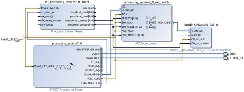
a Cortex-A9 ARM processor of 650 Mhz in the ZYBO ZYNQ XC7Z010-1CLG400C platform.
Figure 7 illustrates the hardware/software codesign approach of the ARM processor and our matrix
inversion architecture.
Figure 7. HW/SW codesign with the matrix inversion as the coprocessor unit.
Considering a 4 × 4 matrix as input of the hardware/software (HW/SW) codesign, the ARM
processor transmits the matrix data to the coprocessor and receives the solution of the matrix inversion.
In this analysis, the time performance was carried out as follows:
tinv = t AXI + tQRD + t BS , (7)
where tinv is the total time for the matrix inversion operation, t AXI is the time intercommunication
between the ARM and FPGA device, tQRD is the time processing of the QRD using PPA systolic cells,
and t BS is the processing time of the back-substitution implementation.
The resulting performance for the implementation is t AXI equal to 0.3369 ms, tQRD = 0.15 ms,
and t BS = 0.17 ms. Therefore, the total time of the parallel matrix inversion is 0.6569 ms. In order
to compare this result, the sequential implementation of the same operation, with only the ARM
processor, was employed achieving 5.0492 ms, which represents a speed up of 7.6864.Electronics 2020, 9, 182 12 of 14
5. Performance Analysis Discussion
As mentioned in Section 1, hardware implementations based on CORDIC strategies need to
carry out several algorithm iterations for converging to the desired results in order to improve the
result accuracy; however, these iterations impact in latency metric (cycles and time), as can be seen in
Table 2, even when high frequency operations are achieved by the state-of-the-art QRD hardwares.
Likewise, the CORDIC-based architectures increase the number of slice registers and slice LUTs.
On the other hand, our proposed architecture decreases the number of slice registers, slice LUTs,
and latency cycles in the design. It only takes a latency of 7 clock cycles for carrying out the QRD
and 5 clock cycles for computing the back-substitution algorithms, which is equivalent to 100 ns and
71.4 ns for a frequency operation of 70 MHz and 77.7 ns and 55.5 ns for a frequency operation of
90 MHz, respectively. As can be observed in Table 2, our proposed matrix inversion architecture is the
fastest architecture, which improves the time performances reported in the open literature. However,
these outstanding advantages are paid by increasing the number of DSP48 elements in the architecture,
which can be balanced by implementing them via slice registers and slice LUTs along the synthesis
process or by using other design strategies in order to reduce the number of DSP48 elements [30].
Finally, the proposed matrix inversion architecture in this paper offers a well-balanced improvement
in the design, achieving high throughput and less hardware resource utilization in comparison of
state-of-the-art FPGA-based architectures.
6. Conclusions
In this paper, a new design of a hardware matrix inversion architecture was presented.
The proposal is based on the QR matrix decomposition and the back-substitution algorithm, which are
implemented using a systolic hardware architecture that requires the RSR operation computed by
a hybrid piecewise polynomial approximation. The results show that the hardware resources and the
time execution are significantly reduced in comparison with the proposals that employ CORDICs and
LUTs. In particular, the experimental results for Virtex-6 technology pointed out that the proposal has
the capacity to compute 7.51 MM/s when 4 × 4 matrices are processed using 12 clock cycles for the
complete matrix inversion operation. Moreover, the SQNR achieved is 58 dB with 16 bit word length.
Under this perspective, the authors consider that this proposal of a fast hardware architecture for the
matrix inversion can be used as a coprocessor in a hardware and software codesign paradigm for
many applications like receivers in MIMO space–time communications and matrix signal processing
applications, where efficient and real-time computations are required.
Author Contributions: Conceptualization, J.V.-C., A.C.-A., R.C.-A., O.L.-G.; Formal analysis, R.C.-A., J.V.-C.,
O.L.-G.; Investigation, O.L.-G., J.O.-A.; Methodology, R.C.-A., J.V.-C., O.L.-G., A.C.-A.; Project administration,
J.V.-C., R.C.-A.; Validation, O.L.-G., J.O.-A.; Writing—original draft, J.V.-C., R.C.-A., A.C.-A., O.L.-G., J.O.-A.;
Writing—review and editing, J.V.-C., R.C.-A., A.C.-A., O.L.-G., J.O.-A. All authors have read and agreed to the
published version of the manuscript.
Funding: This work was financed by the Mexican Ministry of Education (SEP-PRODEP-2019) and by the Mexican
Council for Science and Technology (CONACYT) through the SEP-CONACYT Basic Research Program: Project
reference #241272.
Conflicts of Interest: The authors declare no conflict of interest.
References
1. Castillo-Atoche, A.; Torres-Roman, D.; Shkvarko, Y. Towards real time implementation of reconstructive
signal processing algorithms using systolic arrays coprocessors. J. Syst. Archit. 2010, 56, 327–339. [CrossRef]
2. Liu, C.; Xing, Z.; Yuan, L.; Tang, C.; Zhang, Y. A Novel Architecture to Eliminate Bottlenecks in a Parallel
Tiled QRD Algorithm for Future MIMO Systems. IEEE Trans. Circuits Syst. II Express Briefs 2017, 64, 26–30.
[CrossRef]
3. Chen, W.; Li, F.; Peng, Y. 3D-MIMO Channel Estimation under Non-Gaussian Noise with Unknown PDF.
Electronics 2019, 8, 316. [CrossRef]Electronics 2020, 9, 182 13 of 14
4. Alwan, N.A. Systolic parallel architecture for brute-force autoregressive signal modeling. Comput. Electr. Eng.
2013, 39, 1358–1366. [CrossRef]
5. Skalicky, S.; Lopez, S.; Lukowiak, M. Performance modeling of pipelined linear algebra architectures on
FPGAs. Comput. Electr. Eng. 2014, 40, 1015–1027. [CrossRef]
6. Datta, B.N. Numerical Methods for Linear Control Systems: Design and Analysis; Elsevier: Amsterdam,
The Netherlands, 2004.
7. Higham, N.J. Accuracy and Stability of Numerical Algorithms, 2nd ed.; Society for Industrial and Applied
Mathematics: Philadelphia, PA, USA, 2002.
8. Aslan, S.; Niu, S.; Saniie, J. FPGA implementation of fast QR decomposition based on givens rotation.
In Proceedings of the 2012 IEEE 55th International Midwest Symposium on Circuits and Systems (MWSCAS),
Boise, ID, USA, 5–8 August 2012; pp. 470–473.
9. Muñoz, S.D.; Hormigo, J. High-Throughput FPGA Implementation of QR Decomposition. IEEE Trans.
Circuits Syst. II Express Briefs 2015, 62, 861–865. [CrossRef]
10. Abels, M.; Wiegand, T.; Paul, S. Efficient FPGA implementation of a high throughput systolic array
QR-decomposition algorithm. In Proceedings of the 2011 Conference Record of the Forty Fifth Asilomar
Conference on Signals, Systems and Computers, Pacific Grove, CA, USA, 6–9 November 2011; pp. 904–908.
11. Chen, D.; Sima, M. Fixed-Point CORDIC-Based QR Decomposition by Givens Rotations on FPGA.
In Proceedings of the 2011 International Conference on Reconfigurable Computing and FPGAs, Cancun,
Mexico, 30 November–2 December 2011; pp. 327–332.
12. Bag, J.; Roy, S.; Dutta, P.K.; Sarkar, S.K. Design of a DPSK Modem Using CORDIC Algorithm and Its FPGA
Implementation. IETE J. Res. 2014, 60, 355–363. [CrossRef]
13. Chervyakov, N.; Lyakhov, P.; Babenko, M.; Nazarov, A.; Deryabin, M.; Lavrinenko, I.; Lavrinenko, A.
A High-Speed Division Algorithm for Modular Numbers Based on the Chinese Remainder Theorem with
Fractions and Its Hardware Implementation. Electronics 2019, 8, 261. [CrossRef]
14. Auger, F.; Lou, Z.; Feuvrie, B.; Li, F. Multiplier-Free Divide, Square Root, and Log Algorithms [DSP Tips
and Tricks]. IEEE Signal Process. Mag. 2011, 28, 122–126. [CrossRef]
15. Mahapatra, C.; Mahboob, S.; Leung, V.C.M.; Stouraitis, T. Fast Inverse Square Root Based Matrix Inverse
for MIMO-LTE Systems. In Proceedings of the 2012 International Conference on Control Engineering and
Communication Technology, Liaoning, China, 7–9 December 2012; pp. 321–324.
16. Pizano-Escalante, L.; Parra-Michel, R.; Castillo, J.V.; Longoria-Gandara, O. Fast bit-accurate reciprocal
square root. Microprocess. Microsystems 2015, 39, 74–82. [CrossRef]
17. Aguilera-Galicia, C.R.; Longoria-Gandara, O.; Pizano-Escalante, L.; Vázquez-Castillo, J.; Salim-Maza, M.
On-chip implementation of a low-latency bit-accurate reciprocal square root unit. Integration 2018, 63, 9–17.
[CrossRef]
18. Zhang, C.; Liang, X.; Wu, Z.; Wang, F.; Zhang, S.; Zhang, Z.; You, X. On the Low-Complexity,
Hardware-Friendly Tridiagonal Matrix Inversion for Correlated Massive MIMO Systems. IEEE Trans. Veh.
Technol. 2019, 68, 6272–6285. [CrossRef]
19. Trejo-Arellano, J.; Vázquez Castillo, J.; Longoria-Gandara, O.; Carrasco-Alvarez, R.; Gutiérrez,
C.; Castillo Atoche, A. Adaptive segmentation methodology for hardware function evaluators.
Comput. Electr. Eng. 2018, 69, 194–211. [CrossRef]
20. Kim, S.; Yun, U.; Jang, J.; Seo, G.; Kang, J.; Lee, H.N.; Lee, M. Reduced Computational Complexity Orthogonal
Matching Pursuit Using a Novel Partitioned Inversion Technique for Compressive Sensing. Electronics 2018,
7, 206. [CrossRef]
21. Langhammer, M.; Pasca, B. High-Performance QR Decomposition for FPGAs. In Proceedings of the
2018 ACM/SIGDA International Symposium on Field-Programmable Gate Arrays, Monterey, CA, USA,
25–27 February 2018; pp. 183–188.
22. Ellaithy, D.M.; El-Moursy, M.A.; Zaki, A.; Zekry, A. Dual-Channel Multiplier for Piecewise-Polynomial
Function Evaluation for Low-Power 3-D Graphics. IEEE Trans. Very Large Scale Integr. (VLSI) Syst. 2019,
27, 790–798. [CrossRef]
23. Golub, G.; Van Loan, C. Matrix Computations; Johns Hopkins University Press: Baltimore, MD, USA, 2012.
24. Lee, D.U.; Cheung, R.; Luk, W.; Villasenor, J. Hierarchical Segmentation for Hardware Function Evaluation.
IEEE Trans. Very Large Scale Integr. (VLSI) Syst. 2009, 17, 103 –116. [CrossRef]
25. Kung, S.Y. VLSI Array Processors; Prentice Hall: Upper Saddle River, NJ, USA, 1988.Electronics 2020, 9, 182 14 of 14
26. Parhi, K.K. VLSI Digital Signal Processing Systems: Design and Implementation, 1st ed.; Wiley-Interscience:
Hoboken, NJ, USA, 1999.
27. Canche Santos, L.; Castillo Atoche, A.; Vázquez Castillo, J.; Longoria-Gándara, O.; Carrasco Alvarez, R.;
Ortegon Aguilar, J. An improved hardware design for matrix inverse based on systolic array QR
decomposition and piecewise polynomial approximation. In Proceedings of the 2015 International
Conference on ReConFigurable Computing and FPGAs (ReConFig), Mexico City, Mexico,
7–9 December 2015; pp. 1–6.
28. Cheung, R.; Lee, D.U.; Luk, W.; Villasenor, J.D. Hardware Generation of Arbitrary Random Number
Distributions From Uniform Distributions Via the Inversion Method. IEEE Trans. Very Large Scale Integr.
(VLSI) Syst. 2007, 15, 952–962. [CrossRef]
29. Alimohammad, A.; Fard, S.F.; Cockburn, B.F. A Unified Architecture for the Accurate and High-Throughput
Implementation of Six Key Elementary Functions. IEEE Trans. Comput. 2010, 59, 449–456. [CrossRef]
30. Pushpangadan, R.; Sukumaran, V.; Innocent, R.; Sasikumar, D.; Sundar, V. High Speed Vedic Multiplier for
Digital Signal Processors. IETE J. Res. 2009, 55, 282–286. [CrossRef]
c 2020 by the authors. Licensee MDPI, Basel, Switzerland. This article is an open access
article distributed under the terms and conditions of the Creative Commons Attribution
(CC BY) license (http://creativecommons.org/licenses/by/4.0/).You can also read