GEE Timeseries Explorer - Release 1.1 Andreas Rabe, Philippe Rufin
←
→
Page content transcription
If your browser does not render page correctly, please read the page content below
GEE Timeseries Explorer
                     Release 1.1

    Andreas Rabe, Philippe Rufin

                       Sep 29, 2021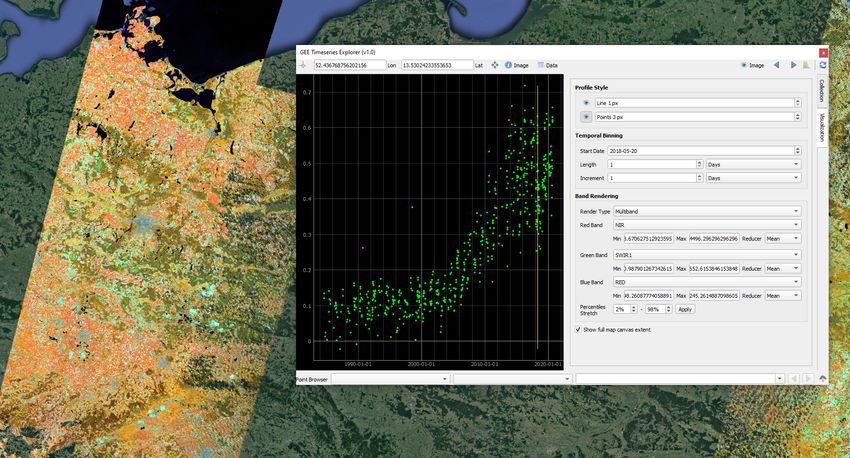
CONTENT

1   GEE Timeseries Exlorer                                                                                                                                                                                    3
    1.1 Installation . . . . .   .   .   .   .   .   .   .   .   .   .   .   .   .   .   .   .   .   .   .   .   .   .   .   .   .   .   .   .   .   .   .   .   .   .   .   .   .   .   .   .   .   .   .    3
    1.2 Getting started . . .    .   .   .   .   .   .   .   .   .   .   .   .   .   .   .   .   .   .   .   .   .   .   .   .   .   .   .   .   .   .   .   .   .   .   .   .   .   .   .   .   .   .   .    4
    1.3 Advanced Usage . .       .   .   .   .   .   .   .   .   .   .   .   .   .   .   .   .   .   .   .   .   .   .   .   .   .   .   .   .   .   .   .   .   .   .   .   .   .   .   .   .   .   .   .   10
    1.4 Contact . . . . . . .    .   .   .   .   .   .   .   .   .   .   .   .   .   .   .   .   .   .   .   .   .   .   .   .   .   .   .   .   .   .   .   .   .   .   .   .   .   .   .   .   .   .   .   12

                                                                                                                                                                                                              i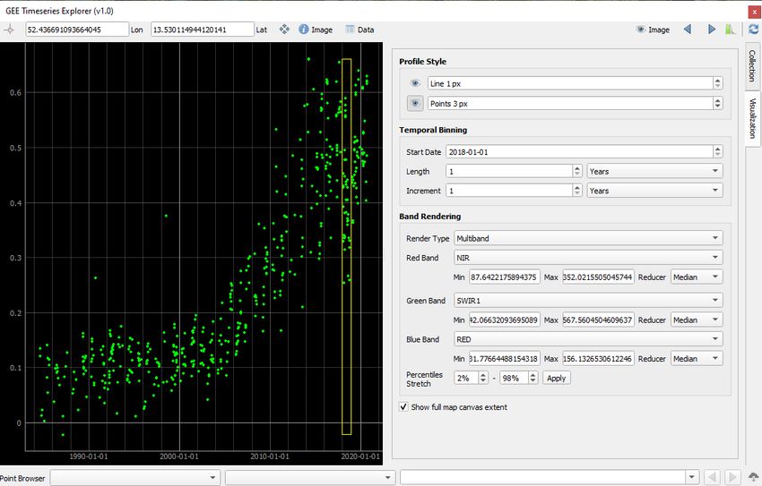
ii
GEE Timeseries Explorer, Release 1.1

This documentation is structured as follows:

CONTENT                                                                           1
GEE Timeseries Explorer, Release 1.1

2                                      CONTENT
CHAPTER

                                                                                                             ONE

                                                                    GEE TIMESERIES EXLORER

GEE Timeseries Exlorer is a QGIS plugin for interactive exploration of temporal raster data available via the
Google Earth Engine (GEE) Data Catalog.
The GEE Timeseries Exlorer plugin adds a panel for selecting a GEE image collection and a plot widget for visualizing
temporal profiles.

1.1 Installation

In QGIS select QGIS > Plugins > Manage and Install Plugins. . . , search for GEE Timeseries Exlorer and install the
plugin.
Note: this plugin relies on the Earth Engine Python API. Search for Google Earth Engine and install this plugin as
well. You may also want to have a look here in case of any issue whilst installing: https://gee-community.github.io/
qgis-earthengine-plugin/ In order to access Earth Engine, you must first authorize your Google account for the use of
the python API. This in turn requires a Google Account with access to Earth Engine.
    • In QGIS select QGIS > Settings > User Profiles > Open Active Profile Folder
    • Navigate to python > plugins > ee_plugin > extlibs_windows (_linux / _darwin on Linux/Mac systems re-
      spectively) and copy the full path to this directory
    • Open the OSGeo4W Shell / Terminal and run the following:

py3_env
python
import sys
sys.path.append(r"Paste path to directory here")
import ee
ee.Authenticate()

Follow the instructions in your browser and copy the authentication code into the OSGeo4W / Terminal.

                                                                                                                   3
GEE Timeseries Explorer, Release 1.1
1.2 Getting started
Overview In the toolbar click to show the GEE Timeseries Exlorer panel.
There are two main panels: The Plot Window on the left and the Collection and Visualization settings on the
right.
Load a Collection The Collection tab on the right panel allows you to select a predefined Image Collection from
the list and filter it by time interval and/or metadata properties. The subsection Collection Editor provides the
python code used to access the imagery and enables full control on the code executed by the user, having access
to the entire Earth Engine Data Catalogue (https://developers.google.com/earth-engine/datasets).
For a quick start, the code snippet for accessing the USGS Landsat 8 Surface Reflectance Tier 1 image collection
is already prepared.
Click on the info button next to the collection list to open and inspect the USGS Landsat 8 Surface
Reflectance Tier 1 description.
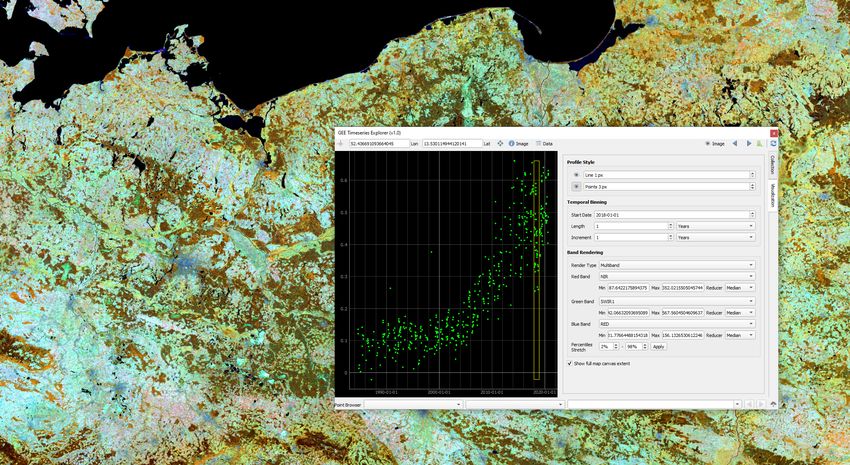
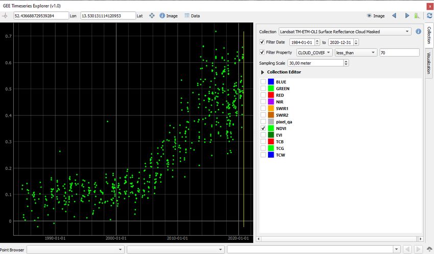
Visualize Time Series This section displays the spectral time series of the user defined collection and time frame.
Click on Activate point selection tool in the upper left corner of the plugin and select at least one spectral band
from the list. Here we use the predefined collection Landsat TM-ETM-OLI Surface Reflectance Cloud Masked
4 Chapter 1. GEE Timeseries ExlorerGEE Timeseries Explorer, Release 1.1
which combines the Landsat sensors into one collection and applies masking based on quality bands (hint: check
the Collection Editor for details). Set Filter Date to 1984-01-01 to 2020-12-31 to make use of the entire
Landsat archive. Furthermore it can be useful to edit Filter Property to only consider scenes with less than 70%
cloud cover.
Then, click into the map canvas to select a point location and to read the temporal profile data.
When changing the date range or filtered metadata properties, click on Read point profile to re-read the current
location.
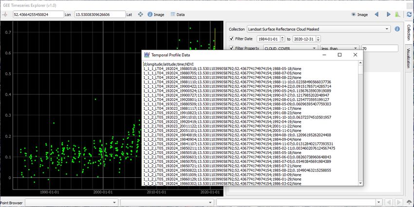
In the top panel, click on to retrieve the displayed time series as raw data:
It provides access to the raw data with information on the unique image id, the geographic coordinates, the date
of acquisition and the spectral values for all bands selected.
Visualize Single Images Apart from plot based time series, you can visualize entire images and image aggregates.
Open the Visualization tab on the right panel. In the subsection Temporal Binning you can specify a temporal
window for which the visualisation will be rendered. By default, this corresponds to a single date, but can be
expanded to a date range by increasing the Length parameters value and/or type (Day, Month, Year). The yellow
vertical line (single date) or box (multi date) in the Plot Window illustrates the given choice graphically and can
further be used to change the temporal window interactively by clicking inside the plot window.
Secondly, select the desired image visualization in the Band Rendering subsection. For RGB composites use
Multiband as Render Type and select an input band for each color channel, e.g by selecting SWIR2 as red band,
NIR as green band and RED as blue band. By default, the Min / Max values are estimated using percentiles
(default: 2% to 98%). Furthermore, we checked Show full map canvas extent to visualize all scenes acquired on
the specified date that fall into our current map canvas extent.
Lastly, click Apply to estimate the values and make sure the image visibility is toggled on .
Also try to use the buttons in the upper right corner of the plugin to jump to the previous/next obser-
vation dates or time frames.
Visualize Temporally Aggregated Images In case of Landsat data it is usefull to not only visualize data at a specific
date in time, but to aggregate multiple observations over a date range (e.g. the revisiting time of 16 days) and to
also visualize observations from neighbouring overflight pathes at the same time. Furthermore, the aggregation
of time series into pixel based statistics is usefull for preserving variance whilst reducing the dimensionality of
the data. Pixel-based calculations over time are referred to as Reducers in Earth Engine. For each band, you can
select from a variety of statistical reducers and visualize them accordingly.
For example, let’s visualize the median of the selected band combination for our entire map canvas using all
imagery acquired in 2018:
Download Time Series Data Often we need time series of spectral bands or indices for multiple locations in space.
GEE-TSE allows to specify a point layer that is loaded in QGIS for which the time series of the selected bands
and time frame can be downloaded to csv-files. To do so, select a point layer as input in the Point Browser panel
at the bottom of the plugin and click in the lower right corner. Specify a target folder in which the .csv-files
for each feature of the point layer are stored.
Furthermore, you can select attributes of the point layer and use the list or the buttons to reload the
plot and image visualization for the given feature.
1.2. Getting started 5GEE Timeseries Explorer, Release 1.1 6 Chapter 1. GEE Timeseries Exlorer
GEE Timeseries Explorer, Release 1.1

1.2. Getting started                                      7
GEE Timeseries Explorer, Release 1.1

8                                      Chapter 1. GEE Timeseries Exlorer
GEE Timeseries Explorer, Release 1.1

1.2. Getting started                                      9
GEE Timeseries Explorer, Release 1.1

1.3 Advanced Usage

Collection Editor In the Collection tab, the subsection Collection Editor provides the python code used to access
      the imagery and enables full control on the code executed by the user. For instance, we might want to filter the
      specified collection prior to plotting and visualization.

                                                                                          images/gee_catalogue.PNG

      Have a look at the datasets available in the Earth Engine Catalogue by clicking on                . For now,
      consider the MOD13Q1 16-day vegetation index product (https://developers.google.com/earth-engine/datasets/
      catalog/MODIS_006_MOD13Q1). Open the Collection Editor and provide python code that loads the collec-
      tion and applies a user-defined cloud masking function. Important: The variable name of the final ImageCol-
      lection must be imageCollection in order to be understood by the plugin.

import ee

# function to mask clouds
def maskClouds(image):
  QA = image.select('SummaryQA')
  return image.updateMask(QA.eq(0))

# define imgcol with selected bands and apply cloud masking
imageCollection = ee.ImageCollection('MODIS/006/MOD13Q1')\
     .select('NDVI','EVI','SummaryQA')\
     .map(maskClouds)

10                                                                         Chapter 1. GEE Timeseries Exlorer
GEE Timeseries Explorer, Release 1.1
In the Collection Editor this then looks as follows:
More Collections Sentinel-2
This collection returns the merged Sentinel-2A and -2B L2A (surface reflectance product) archives. It uses an
aggressive cloud masking discarding images with >50% cloud cover, uses the scene classification layer to remove
saturated pixels, clouds at all confidence levels, cirrus clouds, cloud shadows and snow. Furthermore, the cloud
displacement index (CDI; see Frantz et al. 2018 https://doi.org/10.1016/j.rse.2018.04.046 for details) is used to
improve cloud masking. The collection returns renamed bands and includes a NDVI band for convenience.
import ee
def maskS2scl(image):
scl = image.select('SCL')
sat = scl.neq(1)
shadow = scl.neq(3)
cloud_lo = scl.neq(7)
cloud_md = scl.neq(8)
cloud_hi = scl.neq(9)
cirrus = scl.neq(10)
snow = scl.neq(11)
return image.updateMask(sat.eq(1)).updateMask(shadow.eq(1)).updateMask(cloud_lo.
˓→eq(1)).updateMask(cloud_md.eq(1)).updateMask(cloud_hi.eq(1)).updateMask(cirrus.eq(1)).
˓→updateMask(snow.eq(1)))
def maskS2cdi(image):
cdi = ee.Algorithms.Sentinel2.CDI(image)
return image.updateMask(cdi.gt(-0.8)).addBands(cdi)
bands = ee.List(['B2', 'B3', 'B4', 'B5', 'B6', 'B7', 'B8', 'B8A', 'B11', 'B12', 'QA60',
˓→'SCL', 'cdi'])
(continues on next page)
1.3. Advanced Usage 11GEE Timeseries Explorer, Release 1.1
(continued from previous page)
band_names = ee.List(['blue', 'green', 'red', 'rededge1', 'rededge2', 'rededge3', 'nir',
˓→'broadnir', 'swir1', 'swir2', 'QA60', 'SCL', 'CDI'])
sen = ee.ImageCollection('COPERNICUS/S2_SR')\
.filter(ee.Filter.lt('CLOUDY_PIXEL_PERCENTAGE', 50))\
.map(maskS2scl) \
.map(maskS2cdi) \
.select(bands, band_names)
sen = sen.map(lambda image: image.addBands(image.normalizedDifference(['broadnir', 'red
˓→'])\
.multiply(10000).toInt16().rename('ndvi')))
imageCollection = sen
1.4 Contact
Please provide feedback to Andreas Rabe (andreas.rabe@geo.hu-berlin.de) or create an issue.
12 Chapter 1. GEE Timeseries ExlorerYou can also read