ESB 6th Floor Reverberation Time Study
←
→
Page content transcription
If your browser does not render page correctly, please read the page content below
Eric Egner

Phys 199

12/14/07

                 ESB 6th Floor Reverberation Time Study
Introduction
         As a musician myself, I have had the misfortune of playing in some, quite frankly, terrible places.
Whether it be someone’s basement, a bar, or even places supposedly designed for musical events, these
rooms all posed problems in, but not limited to, two major areas: the reverberation and absorption of
sound. While playing in one of these places, the reverberating sound of what I had previously played
would be so horrible that keeping tempo with my band (I’m a drummer) became a rather painful and
daunting task. So after professor Errede gave a lecture on room acoustics, I decided that for my final
project I would conduct an experiment relating sound’s reverberation time and frequency for a specific
room.

The Experiment
        The original intention was to conduct this experiment in a lecture or concert hall. However, it
proved incredibly problematic to find time in between already scheduled activities (tests and concerts)
to do so. So I settled on running a test in the hallway on the 6th floor of the engineering sciences
building. The hallway, although seemingly not interesting with regard to its acoustical properties, is
square shaped wrapping around an elevator shaft(i.e. has no beginning or end, continuous), with lab
rooms located along its outside perimeter.

        After deciding on a location, it came to my attention that reverberation time can be measured in
multiple ways. One way consists of an impulse sound, such as a gunshot, being recorded then analyzed.
The other method consists of filling up a room with a given frequency of sound, turning off the sound
source, and then analyzing a recording of the process. Wanting to study frequency in relation to
reverberation time, as stated earlier, I went with the steady sound source method.

         In order not to disturb any other people on 6th floor of the ESB, me and Professor Errede went in
late at night to run this experiment. We used a pure sine‐wave function generator connected to a
speaker(pointed down one direction of the hallway) to load the hallway with a standing wave ( note: the
data suggests way more complex wave patterns than simple standing waves, but for all intensive
purposes they will be referred to as standing waves throughout this experiment). We then turned on a
digital recorder which was connected to a dynamic microphone (its properties will discussed later), in
order to capture the sound. After turning on the digital recorder, the sound source was then abruptly
cut out by means of hitting the function generator’s output off button. The resulting reverberating
sound was recorded. We then repeated this process four more times for a total of five different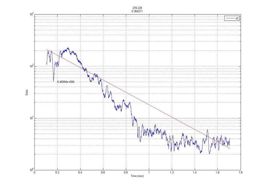
frequencies: 100Hz, 200Hz, 500Hz, 1KHz, 2KHz. (note: thanks to professor Errede for providing his time
and equipment for this experiment)
However, very shortly after looking at the data, we noticed some flaws. All of the data sets had
an unusual spike in the sounds intensity right when the function generator was turned off. Professor
Errede assured me that these “glitch noises” were a result of turning off the function generator to shut
off the sound source. As a result the experiment was repeated in the same exact fashion, except when
in came time to turn off the sound source, we found simply pulling out the cord that connects the
function generator to the speaker, on the end that is connected to the speaker, yielded far more useful
results than the previous method.
The Data
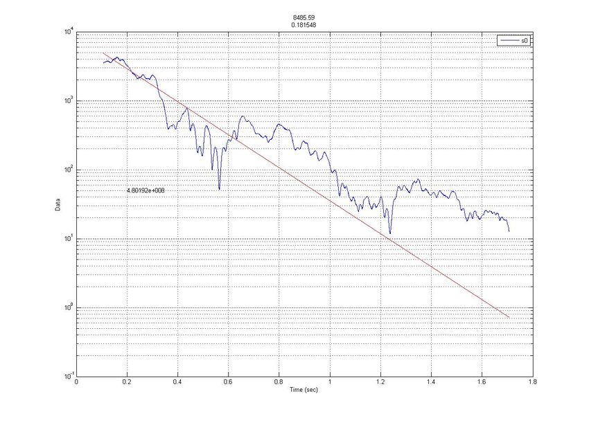
(Note: 2‐D graphs show a semi‐log scale of sound pressure(Y) vs. time (sec)(X)
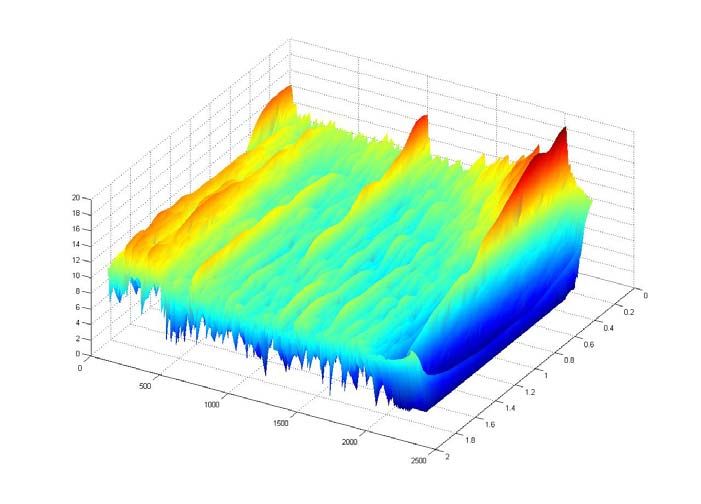
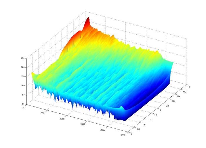
(Note:3‐D graphs show semi‐log scale of sound pressure(Y) vs. frequency(Hz)(X) vs. Time (sec )(Z)
100Hz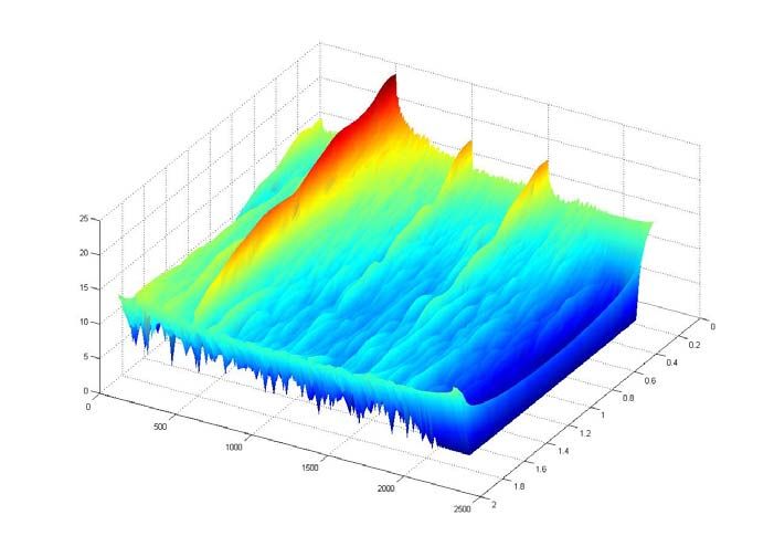
200Hz
500Hz
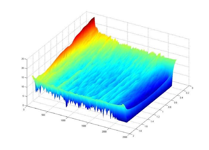
1KHz
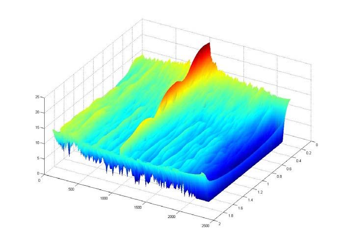
2KHz
Calculations and Analysis
        A few things need to be defined before accurately evaluating the data. The goal is this is to find
the reverberation time for the hallway for each of the five frequencies. The reverberation time is
defined as the amount of time it takes for a sound to decay to one‐millionth of its original intensity (this
is equivalent to a decrease in the sound pressure level of 60 deci‐Bels). This reverberation time will be
dubbed T60 throughout these calculations. Associated with this T60 value, is also a value know as T30
(the time its takes for the sound pressure level to drop 30 deci‐Bels) which is simply half of T60. The
sound pressure level of something can be defined using the following equation.

                                   SPL ≡ 10 log10 ( p 2 po2 )
Where P^2/Po^2 equals the root‐mean‐square of sound over the associated pressure amplitude

The voltage of the dynamic microphone used in this experiment responds linearly to the pressure it
receives when recording.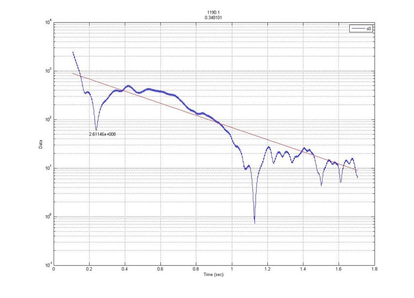
SPL = 10 log10 ( p 2 po2 ) = 10 log10 (Vmic
                                                      2    2
                                                         Vmic o)

  So a simple substitution can relate the sound pressure level to the voltage amplitude of the dynamic
   microphone used. (Note: V mic o= the dynamic microphones calibration to the threshold of human
            hearing, or the voltage amplitude associated with 2 x 10^‐5 pascals of pressure)

        We used a MATLAB (a sound wave analyzing program structure) program dubbed trvb_Studies
to analyze the digital recordings from the dynamic microphone in the experiment. The program uses an
Nth‐order Butterworth digital filter to zero in on a specified frequency (The frequencies in the
experiment: 100, 200, 500, 1000, 2000Hz). When the program analyzes a given sound file and specified
frequency it deviates with relation to the instantaneous amplitude of the microphone voltage over a
said number of samples. Only 51 samples were used over a period of two seconds worth of decaying
sound for each frequency (only two seconds worth of data is needed because the relationship is linear
for pure/standing sine waves). The samples are continuous and adjacent in the duration of the two
second sounds. The program then displays the samples on a semi‐log SPL vs. time plot (the 2‐D graphs)
and shows their relationship to other non‐specified frequencies (3‐D graphs).

        The program finally makes a least‐squares fit to the semi‐log plot (the red line on the graph).
The only data used to make this fit for each plot is the samples taken from .2 to 1.6 seconds. The
program also displays the time decay constant (= τ ) and gives the deviation value (= σ ( t ) ,linearly
proportional to the V mic value), which are both necessary for calculating T30 and T60 times.

                                    σ (t ) = σ o e − t τ
 Since the actual data (not semi‐log plotted) is of exponential decay, this equation can be re‐written to
                   find the respective T30 and T60 times for the five frequency values.

                   T60 = −τ ln (10 −3.0 ) = 6.9078τ
      Now using this table of Decay constants and deviation values from the trvb_Studies program

         Frequency (Hz)                       Deviation value                    Decay Constant (sec)
              100                                 1190.1                              0.348101
              200                                 3794.34                              0.390063
              500                                 2495.78                              0.491387
              1000                                8485.95                              0.181548
              2000                                 278.23                              0.181548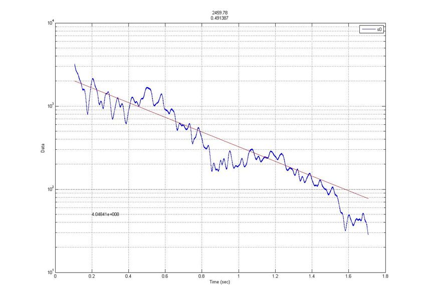
A table of T30 and T60 values can be made

         Frequency (Hz)                       T30 (sec)                                 T60(sec)
               100                              1.202                                    2.405
               200                              1.347                                    2.694
               500                              1.697                                    3.394
              1000                              0.627                                    1.254
              2000                              1.258                                    2.516
(Note: T30 values end up mathematically exactly half of T60 values)

Conclusion
          In conclusion, I was able to calculate the T30 and T60 values from the digital recordings of the
experiment. However, these values do not seem to tell the whole story. The wave forms on the graphs
show another interesting phenomenon. These plots were supposed to digress linearly, but many of
them contain unusual and bizarre waveforms. The explanation lies in two forms of pressure
interference. As stated earlier, the speaker projecting the standing wave was facing down one direction
of the circular hallway on the 6th floor of the ESB. So it is possible that when the sound was abruptly shut
off it created a gap in the projected sound, and because of this, when it came back around the circular
hallway interfered with the sound near the microphone causing various minima in the data (specifically
in the 1000, 2000, and 100 Hz frequencies). Another solution to this problem, known as the flutter echo,
is detailed in Chapter nine of John Backus’ The Acoustical Foundations of Music. In this section he states:

  “An annoying condition can occur in halls when two opposite side walls are flat, and good reflectors of
 sound. In this situation, a sound started between these walls can bounce back and forth between them,
  producing a rapidly repeated echo known as a flutter echo. This condition is quite unadvisable, since it
                               can undesirably emphasize certain frequencies.”

Considering this data set, in which this bizarre interference only occurs mainly in specific frequencies,
and the way the hallway is structured, square with parallel walls, it does a good job of fitting the criteria
for Backus’ flutter echo. However, a more reasonable assumption would be that this flutter echo
combined with the gap of projected sound is what made the data so strange. Of course, more
experiments would be needed to confirm this.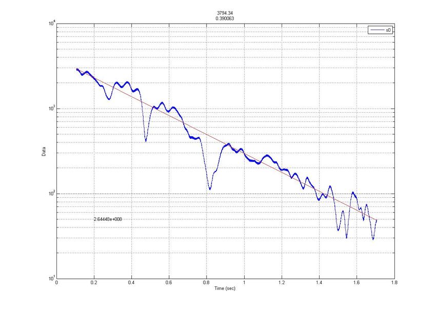
You can also read