Environmental Remote Sensing - GEOG 2021 Lecture 7 Mathematical Modelling in Geography II - UCL Geography
←
→
Page content transcription
If your browser does not render page correctly, please read the page content below
Environmental Remote Sensing
GEOG 2021
Lecture 7

Mathematical Modelling in Geography II
Last time….
• Different types of model
•      statistical, empirical, physically-based, combinations..
• This time some examples
• Simple population growth model

                                                                  2
Simple population growth model
• Require:
– model of population Q as a function of time t i.e. Q(t)
• Theory:
– in a ‘closed’ community, population change given by:
• increase due to births
• decrease due to deaths
– over some given time period t
3
‘Physically-based’ models
• Population change given by:
• increase due to births - decrease due to deaths
• Current population given by:
• Old population + increase due to births - decrease due
to deaths
Q(t t ) Q(t ) births (t ) deaths (t ) [1]
4‘Physically-based’ models
• For period t
– rate of births per head of population is B
– rate of deaths per head of population is D
• So…
births (t ) B * Q(t ) * t
deaths (t ) D * Q(t ) * t [2]
– Implicit assumption that B,D are constant over time t
– So, IF our assumptions are correct, and we can ignore
other things (big IF??)
5Q (t ) Q (t t ) Q (t )
so :
Q (t t ) Q (t )
Q
t
t
births (t ) deaths (t )
t
( B D )Q (t ) [3]
6‘Physically-based’ models
• As time period considered decreases, can write
eqn [3] as a differential equation:
dQ
( B D)Q
dt
• i.e. rate of change of population with time equal to
birth-rate minus death-rate multiplied by current
population
• Solution is ...
7‘Physically-based’ models
Q(t ) Q0e ( BD ) t
• Consider the following:
– What does Q0 mean?
– Does the model work if the population is small?
– How might you ‘calibrate’ the model parameters?
[hint - think logarithmically]
logQt logQ0 B Dt
– What happens if B>D (and vice-versa)?
8‘Physically-based’ models
•So B, D and Q0 all
have ‘physical’
Q(t ) Q0e ( BD ) t
meanings in this
system
Q
B>D
Q0
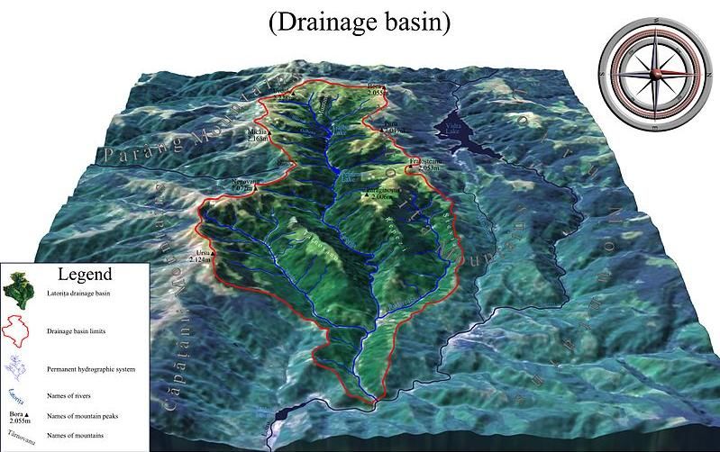
BHydrological (catchment) models
Latoriţa River drainage basin, Romania 10Hydrological (catchment) models
• Want to know water volume in/out of catchment
• Simplest e.g. time-area method not dependent
on space (1D) (lumped model)
• Next level of complexity - semi-distributed
models e.g. sub-basin division
• Spatially distributed i.e. need 2D representation
of catchment area
• More complex still, use full 3D representation of
catchment area, topography, soil types etc.
11Simplest catchment models: time-area hydrograph
• Schematic model
– very simplified, no physics
• Empirical/statistical
– predicts discharge, Q (m3s-1), based on rainfall intensity, i
(mm hr-1), and catchment area, A (m2) i.e. Q = ciA
• c is (empirical) runoff coefficient i.e. fraction of rainfall which
becomes runoff
• c is particular to a given catchment (limitation of model)
– more than one area? Divide drainage basins into isochrones
(lines of equal travel time along channel), and add up….
– Q(t) = c1A1i(t-1) + c2A2i(t-2) + ….. + cnAni(t-n)
12Process-type catchment models
• More complex – some physics
– precipitation, evapotranspiration, infiltration
– soil moisture conditions (saturation, interflow,
groundwater flow, throughflow, overland flow, runoff
etc.)
• From conservation of “stuff” - water balance
equation
– dS/dt = R - E - Q
– i.e. rate of change of storage of moisture in the
catchment system, S, with time t, is equal to inflow
(rainfall, R), minus outflow (runoff, Q, plus
evapotranspiration, E)
– E.g. STORFLO model (in Kirkby et al.)
13http://www.geocomputation.org/1999/042/gc_042.htm
More complex?
• Consider basin morphometry (shape) on runoff
– Slope, area, shape, density of drainage networks
– Consider 2D/3D elements, soil types and hydraulic
properties
• How to divide catchment area?
– Lumped models
• Consider all flow at once... Over whole area
– Semi-distributed
• isochrone division, sub-basin division
– Distributed models
• finite difference grid mesh, finite element (regular, irregular)
– Use GIS to represent - vector overlay of network?
– Time and space representation?
14TOPMODEL: Rainfall runoff
From: http://www.es.lancs.ac.uk/hfdg/topmodel.html
15Very complex: MIKE-SHE
•Name
•Combination of
physical, empirical
and black-box…
•Can “simulate all
major processes in
land phase of
hydrological cycle”
!!
From: http://www.dhisoftware.com/mikeshe/Key_features/ 16Other distinctions
• Analytical
– resolution of statement of model as combination of
mathematical variables and ‘analytical functions’
– i.e. “something we can actually write down”
– Very handy & (usually) very unlikely.
– e.g. biomass = a + b*NDVI
– e.g.
dQ
aQ Q Q0e at
dt
17Other distinctions
• Numerical
– solution to model statement found e.g. by calculating
various model components over discrete intervals
• e.g. for integration / differentiation
18Inversion
• Remember - turn model around i.e. use model to
explain observations (rather than make
predictions)
– Estimate value of model parameters
– E.g. physical model: canopy reflectance, canopy as a
function of leaf area index, LAI
• canopy = f(LAI, …..)
– Inversed: measure reflectance and use to estimate LAI
• LAI = f-1(measured canopy)
19Inversion example: linear regression
• E.g. model of rainfall with altitude
– Y = a + bX +
– Y is predicted rainfall, X is elevation, a and b are constants of
regression (slope and intercept), is residual error
• arises because our observations contain error
• (and also if our model does not explain observed data perfectly e.g.
there may be dependence on time of day, say….)
– fit line to measured rainfall data, correlate with elevation
20Inversion example: linear regression
Y = a + bX
Y (rainfall,mm)
best fit
Y
Intercept, a
X
Slope, b is Y/ X
X (elevation, m)
21Inversion example: linear regression best fit
with
Y (rainfall,mm) outlier
best fit
without
Outlier?
outlier
Y
Intercept, a
X
Slope, b is Y/ X
-ve intercept! X (elevation, m)
22Inversion Y = a + bX +
• Seek to find “best fit” of model to observations
somehow
– most basic is linear least-squares (regression)
– “Best fit” - find parameter values which minimise some error
function e.g. RMSE (root mean square error)
n N
measured mod elled 2
RMSE
n 1 N 1
• Easy if we can write inverse model down (analytical)
• If we can’t …… ?
23Inversion
• Have to solve numerically i.e. using sophisticated trial
and error methods
– Generally more than 1 parameter, mostly non-linear
– Have an error surface (in several dimensions) and want to find
lowest points (minima)
– Ideally want global minimum (very lowest) but can be
problematic if problem has many near equivalent minima
‘Easy’ Hard ‘Easy’
24Inversion
• Have to solve numerically i.e. using sophisticated trial
and error methods
– E.g. Gradient descent
– Quasi-Newton method,
– Simulated Annealing,
– Artificial Neural Networks (ANNs),
– Genetic Algorithms (GAs), etc.
‘Easy’ Hard ‘Easy’
25Inversion
• E.g. of aircraft over airport and organising them to land
in the right place at the right time
– Many parameters (each aicraft location, velocity, time, runway
availability, fuel loads etc.)
– Few aircraft? 1 solution i.e. global minimum & easy to find
– Many aircraft? Many nearly equivalent solutions
– Somewhere in middle? Many solutions but only one good one
‘Easy’ ‘Easy’ ‘Hard’
26Which type of model to use?
• Statistical
– advantages
• simple to formulate & (generally) quick to calculate
• require little / no knowledge of underlying (e.g. physical) principles
• (often) easy to invert as have simple analytical formulation
– disadvantages
• may only be appropriate to limited range of parameter
• may only be applicable under limited observation conditions
• validity in extrapolation difficult to justify
• does not improve general understanding of process
27Which type of model to use?
• Physical/Theoretical/Mechanistic
– advantages
• if based on fundamental principles, more widely applicable
• may help to understand processes e.g. examine role of
different assumptions
– disadvantages
• more complex models require more time to calculate
• Need to know about all important processes and variables
AND write mathematical equations for processes
• often difficult to obtain analytical solution & tricky to invert
28Summary
• Empirical (regression) vs theoretical (understanding)
• uncertainties
• validation
– Computerised Environmetal Modelling: A Practical Introduction Using
Excel, Jack Hardisty, D. M. Taylor, S. E. Metcalfe, 1993 (Wiley)
– Computer Simulation in Physical Geography, M. J. Kirkby, P. S.
Naden, T. P. Burt, D. P. Butcher, 1993 (Wiley)
– http://www.sportsci.org/resource/stats/models.html
29Coursework – Wetland area extend
31Coursework - STELLA
• STELLA 10.0.4
– free 30-day trial
• SFTP to download files
from UCL Geog machines
– Mac: terminal
– Windows: FTP software (e.g. FillZilla)
• Or SFTP commands (e.g. cygwin)
Server: shankly.geog.ucl.ac.uk
32You can also read