Supplement of Identifying uncertainties in hydrologic fluxes and seasonality from hydrologic model components for climate change impact assessments

Supplement of Hydrol. Earth Syst. Sci., 24, 2253–2267, 2020
https://doi.org/10.5194/hess-24-2253-2020-supplement
© Author(s) 2020. This work is distributed under
the Creative Commons Attribution 4.0 License.

Supplement of
Identifying uncertainties in hydrologic fluxes and seasonality from hydro-
logic model components for climate change impact assessments
Dongmei Feng and Edward Beighley

Correspondence to: Dongmei Feng (dmei.feng@gmail.com)

The copyright of individual parts of the supplement might differ from the CC BY 4.0 License.

Hydrologic model development

 The RCM assumes water excess available for surface runoff (es) is proportional to
precipitation rate (P). The proportion is represented by a coefficient value (e.g., 0 to 100%) and
is dependent on land cover, soil and topographic characteristics. The coefficient value is smaller
for dry and flat areas with permeable soils and vegetated surfaces, as compared to that for wet
and steep areas with more impervious areas (e.g., roads, parking lots, roofs). In this work, a dual
runoff-coefficient method is used, which assigns a larger runoff coefficient (C2) to wet soils
(relative soil moisture at upper soil layer U ≥ threshold t) and smaller runoff coefficient (C1) to
dry soils (relative soil moisture U < threshold t) (Eq. (S1)). The water excess available for
subsurface runoff (ess) is a function of saturated hydraulic conductivity (ksat) and relative soil
moisture in lower soil layer (L) (Eq. (S2)).
 = 1 × < 
 (S1)
 = 2 × ≥ 
 
 = _ × ( ) (S2)
 
where es and ess are water excess available for surface and subsurface runoff, respectively, (m d-
1
 ); P is precipitation rate (m d-1); C1 is dry runoff coefficient; C2 is wet runoff coefficient; U and
L are relative soil moisture at upper and lower soil layer, respectively; t is relative soil moisture
threshold differentiating dry and wet soil conditions; is saturated hydraulic conductivity (m
d-1); _ is a scaler; b is Clapp-Hornberger parameter and n is soil porosity. C1, C2, t and
 _ are parameters needing calibration.
 In the VIC algorithm, surface runoff is generated as infiltration excess where the
infiltration rate is characterized by the variable infiltration curve (Wood et al., 1992). In this
work, the framework of modified 2-layer VIC model (VIC-2L) (Liang et al., 1996) is used. The
water excess available for surface runoff is calculated as shown in Eq. (S3)-(S4). The water
excess available for subsurface runoff is a function of soil moisture in lower soil layer (Eq. (S5)),
which is a linear function of soil moisture when the soil is relatively dry and quadratic when the
soil is close to saturation:
 + ∆ 1+ 
 = − ( − )/∆ − ( |0, [1 − ]|) /∆ (S3)
 
 = [1 − (1 − )1⁄ ] (S4)
 2
 |0, L − |
 = L + ( − )( ) (S5)
 − 
where z is soil depth in upper layers (m); s is relative soil moisture at saturation; im is maximum
infiltration capacity (m); i0 is infiltration capacity (m); bi is infiltration curve parameter; A is the
fraction of saturation; DM is maximum base flow (m d-1); DS is the fraction of DM at which the
non-linear base flow begins; WS is the fraction of saturation at which the non-linear base flow
occurs; ∆ is time step (d). bi, DM, DS and WS are parameters which need calibration.

 1

In STP algorithm, the surface runoff is generated as saturation excess overland flow (Eq.
(S6)). The saturation fraction of the catchment fsat is determined as a function of topographic
index (Eq. (S7)-(S8)).
 = ∗ (S6)
 = ∗ ex p( − 0.5 ∇ ) (S7)
where is the fraction of saturated area; is a decay factor for surface runoff water excess
(m-1); ∇ is groundwater table depth (m); is the maximum saturated fraction and is defined
as the percent of grid cells in each sub-basin with a topographic index () that is ≥ the mean 
determined by averaging all grid cell  values:
 
 = ln ( ) (S8)
 ( )
where is the specific catchment area (i.e.,upslope area per unit contour length) and  is the
pixel slope. The specific catchment area and slope  are calculated for grid cell using the
gridded elevation data and the TauDEM tools (Tarboton, 2003).
 The water excess available for subsurface runoff is a function of maximum base flow rate
and groundwater table depth:
 = ∗ ex p( − ∗ ∇ ) (S9)
where is a decay factor for subsurface runoff water excess (m-1), and is the maximum
baseflow rate (m d-1). Water excess for both surface and subsurface runoff are dependent of the
groundwater table depth ∇ . Here, the water table depth ∇ is determined by applying the method
used in (Niu et al., 2005), which assumes the water head at depth z is in equilibrium with that at
ground water depth ∇ (Eq. (S10)-(S13)).
 ( ) − = − ∇ (S10)
where ( ) and are the matric potentials at depth z and at groundwater table depth ∇ (m).
The soil at the groundwater table depth is assumed to be saturated. Based on Clapp-Hornberger
relationship (Clapp and Hornberger, 1978), ( ) can be expressed as:
 ( ) − 
 ( ) = ( ) (S11)
 
where θ(z) and θsat are soil moisture content at depth z and groundwater table depth ∇ ,
respectively, b is a Clapp-Hornberger parameter. By substituting Eq. (S10) with Eq. (S11), the
soil matric profile at depth z can be expressed as:
 − ( ∇ − ) −1/ 
 ( ) = ( ) (S12)
 
 Then, the groundwater table depth ( ∇ ) can be determined by solving Eq.S13 iteratively.
 ∇
 = ∫ ( − ( )) (S13)
 0

where Dθ is the soil moisture deficit, which can be calculated in Eq.S14:

 2

 

 = ∑( − )∇ (S14)
 =1

where is the soil moisture content at the ith soil layer; ∇ is the soil thickness of ith soil layer,
m is the number of soil layer, m=2 in this study. In STP algorithm, fover, fdrain, Qm and φsat are
parameters to be calibrated.

 = min (PET, W − Wmin ) (S15)
where PET is the potential evapotranspiration estimated using the method proposed by
Raoufi and Beighley (2017); W is water content in the upper soil layers; Wmin is the
minimum water content in the soil, defined as 0.15× Ws ; Ws is soil water content as
saturation.

 = × ( ) (S16)
 
 = × ( ) (S17)
 
where K is the water flux from the upper soil layer to the lower soil layer (m d-1); and D is the
water flux transported from the lower soil layer to the upper soil layer due to diffusion (m d-1).
Plane Routing:
 
 + = (S18)
 
 + = (S19)
 
Channel Routing:
 
 + = + (S20)
 
where ys and yss are water depth (or thickness) of surface and subsurface runoff, respectively
(m); qs and qss are surface and subsurface runoff flow rates per unit width of plane (m2 s-1); dxp is
the distance step along the plane (m); AC is the cross section area of flow in the channel (m2); Qc
is the flow rate in channel (m3 s-1); dxc is the distance step along the channel (m); and dt is the
time step (s).

 3

Uncertainty Analysis
 
 = ∑ ( − )2 (S21)
 =1

 . = ∑ ∑ ( − − + )2 (S22)
 =1 =1

 3.4 = − ( + + + + . 
 + . + . + . + . (S23)
 + . )
where is the average of all simulations from the ith hydrologic model with all combinations
of parameter sets, GCMs and RCPs; the average of all simulations from the jth parameter
set with all combinations of hydrologic models, GCMs and RCPs; is the average of all
simulations from the ith hydrologic model and jth parameter set with all combinations of GCMs
and RCPs. Other terms in Eq. (3) can be calculated similarly using Eq. (S20)-(S21).

 6075
 1 ( )
 = ∑ (S24)
 6075 ( )
 =1

where is the average fractional effect of term e (i.e, each of 11 terms in Eq. (3)); ( ) is
the sum of variance of effect e in the mth subsample, and the ( ) is the total variance in
the mth subsample. So in this study, there are 11 values in total, representing the uncertainty
contributions of 11 terms in Eq. (3), with a sum of 1.0.

Probability of estimated changes
Bayesian model averaging (BMA) has been used to infer the probability of a quantity predicted by
an ensemble of models(Duan et al. 2007). The BMA scheme can be described as below:
For a predicted quantity variable y (i.e., the discharge), the probability of predicted y, given the
observation D = (d1, d2, d3,…, dt) and model ensemble M = (m1,m2,m3,…, mK), ( | ) can be
calculated as:
 
 ( | ) = ∑ ( | ) × ( | , ) (S25)
 =1
where k is the model ID and K is the number of models (i.e., K=3×3×10=90, note, the BMA is
performed on historical period (1986-2005), so no RCP is considered); ( | ) is the probability
of model k to be the correct model given the observation D; ( | ) is also called the weight of
model k which is determined by the model’s ability for reproducing the observed values of quantity
y; ( | , ) is the probability that model k generates the prediction of y; here, ( | , ) is
assumed to be normal distribution. If model k predicts a value of , then the probability that model
k generates prediction y is normally distributed with a mean = (known) and standard

 4

deviation (unknown). Therefore, to get the probability of predicted quantity y, the statistics 
and the weights ( | ) need to be determined. If we denote ( | ) as and the unknown
parameters as θ, then
 = { , , = 1,2,3, … } (S26)
The optimal θ should maximize the probability of prediction y. If we denote the cost function as
 ( ):
 
 ( ) = ∑ × ( | , ) (S27)
 =1
To maximize ( ), the Expectation–Maximization (EM) algorithm is used. Details on EM can be
found in (Duan et al. 2007).
 In this study, the annual mean discharge and annual maximum daily discharge are the
considered variables. Since these two variables are not normally distributed, a Box-Cox
transformation is performed before applying the EM method. Considering the GCMs’ predictions
are not temporally consistent with reality (i.e., the GCMs’ prediction does not have correct timing),
the observation and simulation are both ranked from high to low, and then ( ) is maximized based
on the ranked series. The procedure is as follows:
Step I: Calculate the observed annual mean discharge (or annual maximum daily discharge) at
each watershed of interest for the period 1986-2005
Step II: Calculate the simulated annual mean discharge (or annual maximum daily discharge) for
each simulation in the ensemble (3×3×10=90 models) for the same period
Step III: Rank the observed and simulated annual mean discharge (or annual maximum daily
discharge) in a descending order
Step IV: Calculate the Box–Cox coefficient λ for each watershed by using the BoxCox.lambda
function in R and transform the quantities by using Eq.S26:
 − 1
 = (S28)
 
Step V: Apply the EM process to the transformed series and estimate the weights and variance
of all models
Step VI: Calculate the probability of estimated changes in Qm, Qp and Q100 in the future (2081-
2100) relative to 1986-2005 using the weights obtained in Step V

For Qm, the statistics are:
 
 = ∑ , × , (S29)
 =1
 (S30)
 2 2
 = ∑ , × ( , − )
 =1

 5

where and are the mean and standard deviation of posterior distribution of relative
changes in Qm; , is the weight of model k in terms of Qm; , is the relative change in Qm
predicted by model k; K is the total number of models, and here it is 90.
For Qp, the statistics are:
 
 = ∑ , × , (S31)
 =1
 (S32)
 2 = ∑ , × ( , − )2
 =1

where and are the mean and standard deviation of posterior distribution of relative changes
in Qp; , is the weight of model k in terms of Qp; , is the relative change in Qp predicted by
model k.
For Q100, the statistics are:
 
 100 = ∑ , × ,100 (S33)
 =1
 (S34)
 100 2 = ∑ , × ( ,100 − 100 )2
 =1

where 100 and 100 are the mean and standard deviation of posterior distribution of relative
changes in Q100; , is the weight of model k for Qp; ,100 is the relative change in Q100
predicted by model k. Here, the weights for Qp are used because Q100 is estimated based on the
statistics of Qp series, so it is reasonable to assume that the model having a better ability in
reproducing the annual peak discharge should also have a better ability in reproducing the Q100.

 6

7

8

.

 9

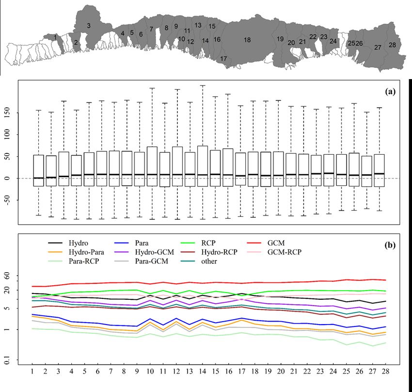
Figure S4. (a) Projected relative changes (%) in annual mean discharge (Qm) in the major
SBC watersheds (indicated by the grey watersheds in the map) during 2081-2100 as
compared to historical period (1986-2005); each bar depicts relative changes in minimum,
maximum, median, 1st and 3rd quartiles for the ensemble outputs; bars from left to right
spatially corresponding to watersheds from west to east. For clarity, only watersheds with
drainage areas larger than 7 km2, which account for roughly 83% of the study area, are
shown. (b) Relative sources (%) of the uncertainties in the projected changes at each of
these watersheds; the category “other” is the uncertainty from the 3rd and 4th orders of
interactions between the 4 major sources (i.e., GCMs, RCPs, Hydrologic models, denoted
by “Hydro” and parameters denoted by “Para”)

 10

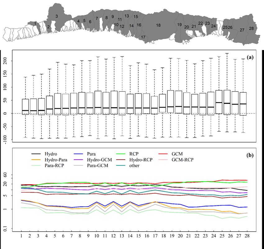
Figure S5. (a) Projected relative changes (%) in annual peak discharge (Qp) in the major
SBC watersheds (indicated by the grey watersheds in the map) during 2081-2100 as
compared to historical period (1986-2005); each bar depicts relative changes in minimum,
maximum, median, 1st and 3rd quartiles for the ensemble outputs; bars from left to right
spatially corresponding to watersheds from west to east. For clarity, only watersheds with
drainage areas larger than 7 km2, which account for roughly 83% of the study area, are
shown. (b) Relative sources (%) of the uncertainties in the projected changes at each of
these watersheds; the category “other” is the uncertainty from the 3rd and 4th orders of
interactions between the 4 major sources (i.e., GCMs, RCPs, Hydrologic models, denoted
by “Hydro” and parameters denoted by “Para”)

 11