"Getting Connected" Technical Assessment - MLA
←
→
Page content transcription
If your browser does not render page correctly, please read the page content below

“Getting Connected”
                       Technical Assessment

Project code:                              B.FLT.8009

Prepared by:                               Kimberley Wockner, Premise Agriculture
                                           David Lamb, University of New England
Date published:                            1 July, 2018

PUBLISHED BY
Meat and Livestock Australia Limited
Locked Bag 1961
NORTH SYDNEY NSW 2059

Appendix 2

Meat & Livestock Australia acknowledges the matching funds provided by the Australian
Government to support the research and development detailed in this publication.

 This publication is published by Meat & Livestock Australia Limited ABN 39 081 678 364 (MLA). Care is taken to ensure the accuracy of the
information contained in this publication. However MLA cannot accept responsibility for the accuracy or completeness of the i nformation or
      opinions contained in the publication. You should make your own enquiries before making decisions concerning your interests.
                    Reproduction in whole or in part of this publication is prohibited without prior written consent of MLA.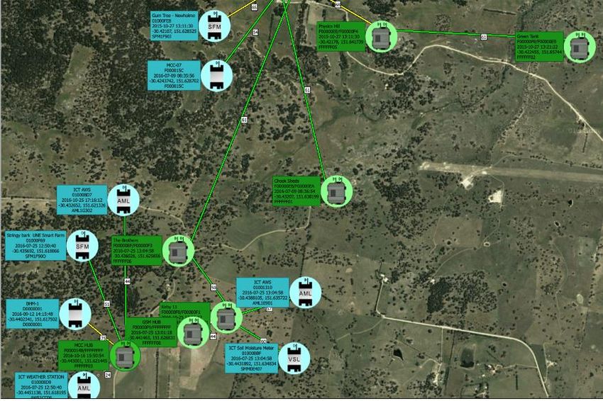
B.FLT.8009 – Getting Connected – Appendix 2

                                               Table of contents
Author Acknowledgment ...................................................................................................... 4
1     Getting connected ......................................................................................................... 4
            Data - bits, packets and bytes ................................................................................. 6
            Moving data and data speeds ................................................................................. 7
2     Internal connectivity - Communicating with devices inside feedlots ............................... 7
            Fibre connectivity .................................................................................................... 7
            Wired connectivity ................................................................................................... 8
            On-farm radio networks – LANs, WLANs and WANs .............................................. 9
      2.3.1       Radio transmission and antennas .................................................................. 10
      2.3.2       Frequency, bandwidth, capacity and speed ................................................... 13
      2.3.3       Transmission power ....................................................................................... 15
      2.3.4       Store and forward telemetry ........................................................................... 16
      2.3.5       Mesh networks............................................................................................... 17
      2.3.6       Long range/lower power WAN– 915 MHz ...................................................... 19
      2.3.7       LORA-WAN ................................................................................................... 20
      2.3.8       Point-to-point links within feedlots .................................................................. 22
3     External connectivity .................................................................................................... 23
            Telecommunications Networks ............................................................................. 23
            Landline - ADSL and ADSL2+............................................................................... 25
            Communicating through the mobile phone network ............................................... 25
      3.3.1       Mobile phone basics ...................................................................................... 26
      3.3.2       Mobile devices and congestion ...................................................................... 30
      3.3.3       Mobile phone coverage for Australian producers ........................................... 32
      3.3.4       The use of cell boosters ................................................................................. 34
      3.3.5       Mobile Roaming ............................................................................................. 35
      3.3.6       Device connectivity and data speeds ............................................................. 36
            Cellular devices in feedlots ................................................................................... 39
      3.4.1       Automatic weather stations ............................................................................ 39
      3.4.2       Safety and performance monitoring systems – telematics.............................. 39
      3.4.3       Positioning and guidance ............................................................................... 41
      3.4.4       Remote vision system utilising the mobile network......................................... 42
      3.4.5       Accessing data and information via the mobile phone network ...................... 43
            Satellite communications options .......................................................................... 45
            The NBN ............................................................................................................... 47
      3.6.1       Fixed wireless ................................................................................................ 48
      3.6.2       Satellite NBN - Sky Muster............................................................................. 49
      3.6.3       Broadband data plans - Speed, capacity and ‘shaping’ .................................. 49

                                                                                                                        Page 2 of 75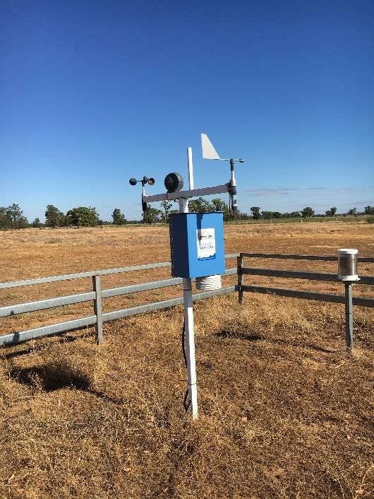
B.FLT.8009 – Getting Connected – Appendix 2

           Tailor-made mobile cells ....................................................................................... 51
           Optical fibre to feedlots ......................................................................................... 52
           Bonded broadband ............................................................................................... 53
4    Second tier telecommunications providers .................................................................. 53
5 A selection of other emerging communications technologies that may make a
difference to feedlot telecommunications .......................................................................... 57
           Deployable networks for transient or moving targets ............................................. 57
           Voice communications over Internet and Wi-Fi (VoWIFI) ...................................... 57
           Narrow band-IoT on the mobile network ............................................................... 58
           Low-cost LEO telecommunications satellites ........................................................ 58
           Increasing data speeds on copper - G.Fast and XG.fast ....................................... 59
6    Emerging technologies for the feedlot industry and implications for connectivity ........ 60
           Smart tags ............................................................................................................ 60
     6.1.1        Example - Provenance4 ................................................................................. 60
     6.1.2        Example - REDI tag ....................................................................................... 62
           Bunk scanners (e.g. Manabotix)............................................................................ 64
7    References ................................................................................................................... 72

                                                                                                                        Page 3 of 75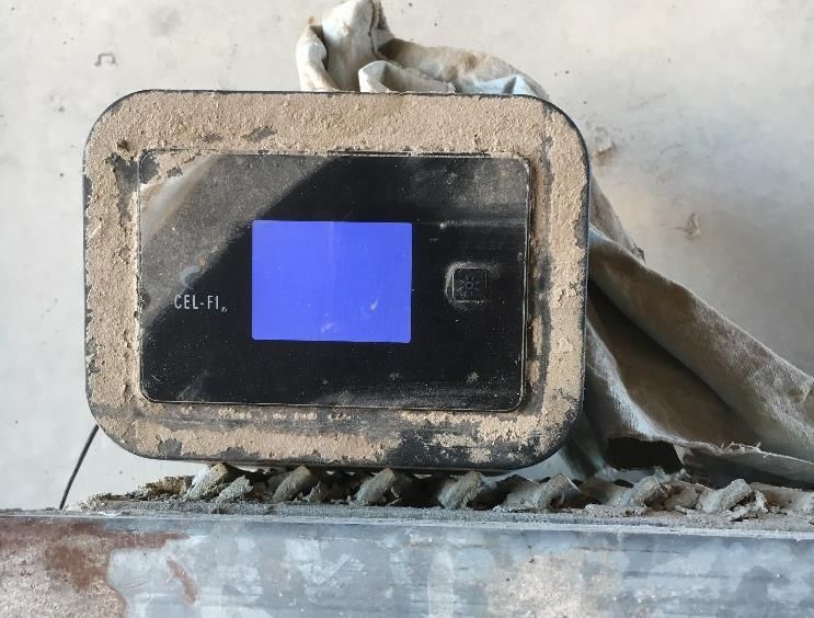
B.FLT.8009 – Getting Connected – Appendix 2

Author Acknowledgment
The authors would like to acknowledge, as a principal source of material for this Appendix, the
report “Accelerating precision agriculture to decision agriculture: A review of on-farm
telecommunications challenges and opportunities in supporting a digital agriculture future for
Australia”. (University of New England and Cotton Research and Development Corporation),
September 2017, 128 pages. ISBN 978-1-921597-74-9 (Hard copy), ISBN 978-1-921597-75-6 (Digital).

1 Getting connected
Feedlots are data and information rich environments, with many potential ‘moving parts’ (Figure
1-1). From a day to day management perspective, the feedlot office is typically the primary interface
between the outside world, of cloud-based services and internet-based decision support tools and
repositories, and the data generating environment of the many moving parts of the feedlot itself.

Connectivity is the key. Here we mean telecommunications connectivity, which takes two forms:
voice connectivity, namely making and receiving phones calls, and data connectivity, taken to mean
exchanging data in its many forms. One has to consider the many sources of data from within a
feedlot to understand the many forms of data that we are referring to here. Data can include
information such as weights taken from a weighbridge, live vision (or still images) transmitted from a
camera located on a weighbridge or in induction sheds or pens, weather measurements
(temperature, humidity, wind etc) from an automatic weather station, remote monitoring systems
on feedlot machinery, control data from an irrigator, water levels in storages and pump pressure,
weight and tag data from an induction shed, and bunk call data at the mill and in the feed truck.
Some of the data is manipulated into information using cloud-based servers and other data is made
accessible via internet (www) access. Of course, the ultimate link in the chain is feedlot staff, mostly
on-the-go, who need to stay in touch with each other and with their operation, both upstream and
downstream, and who are relying upon the many pieces of information that these connected data
sources provide.

Not all of these data sources are in digital form. Paper records still play an important, if not
dominant, role in the Australian feedlot industry (Figure 1-2), reflecting a combination of propensity,
appetite and confidence of feedlot operators to move into a digital age. In many cases, paper
records are simply the only option, as connectivity, that all important roadway of moving digital data
around, is simply not available.

                                                                                                Page 4 of 75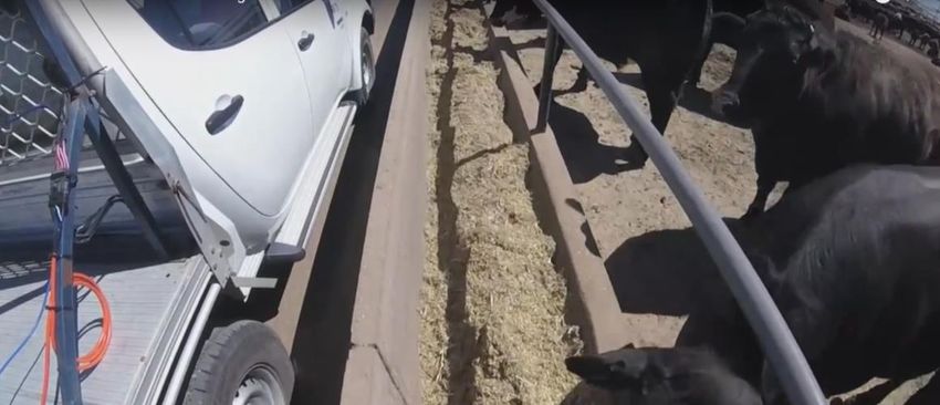
B.FLT.8009 – Getting Connected – Appendix 2

Figure 1-1. Some of the many data/information sources and consumers in a feedlot environment

                                                                                                       Page 5 of 75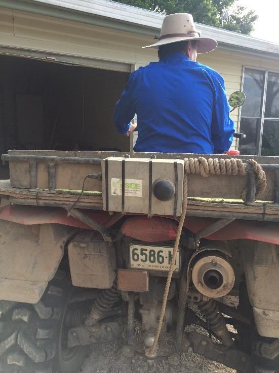
B.FLT.8009 – Getting Connected – Appendix 2

Figure 1-2. Paper records play an important, and currently dominant, role in the operations of many Australian feedlots.

For the purposes of understanding and discussing connectivity, as it relates to Australian feedlots,
we will consider separately ‘external’ and ‘internal’ connectivity. In this document, external
connectivity refers to connecting people and devices directly to the outside world. Note the
emphasis on ‘directly’; in other words, involving a single link. This could include using the mobile
phone for example from inside the feedlot, or a device that transmits data directly to the ‘cloud’
(again, say via a mobile phone link). Internal connectivity is taken to mean connectivity links that
exist inside the feedlot, and where relevant, the associated farm precinct. This may involve one or
two steps. Ultimately the device, or person that is connected internally, may end up connected
(externally) to the outside world. However, in many cases the internal connectivity utilises different
link technology to that utilised by devices (externally) linked directly to the outside world.

       Data - bits, packets and bytes
Just as atoms are the fundamental building blocks of all matter (including us), data also has a basic
building block - the bit. This smallest unit of data is a binary digit (bit is short for ‘binary digit’) which
is either a ‘one’ (1) or a ‘zero’ (0). A data packet is the smallest data package (a combination of 1’s
and 0’s) that is conveyed, from one location to the next, via a network. The packet conveys the basic
information which may include identification, status of connection and structure of message
(contained in the packet). A data packet may range in size from only a few bits through to 64,000
bits (64 kbits) depending on the information to be conveyed and the type of network it is to be
conveyed along. A group of 8 bits is typically utilised as a single unit, known as a byte where 1 byte =
8 bits. Typically, computers use a byte, that is a string of 8 bits, to represent a character such as a
letter, number or symbol.

                                                                                                             Page 6 of 75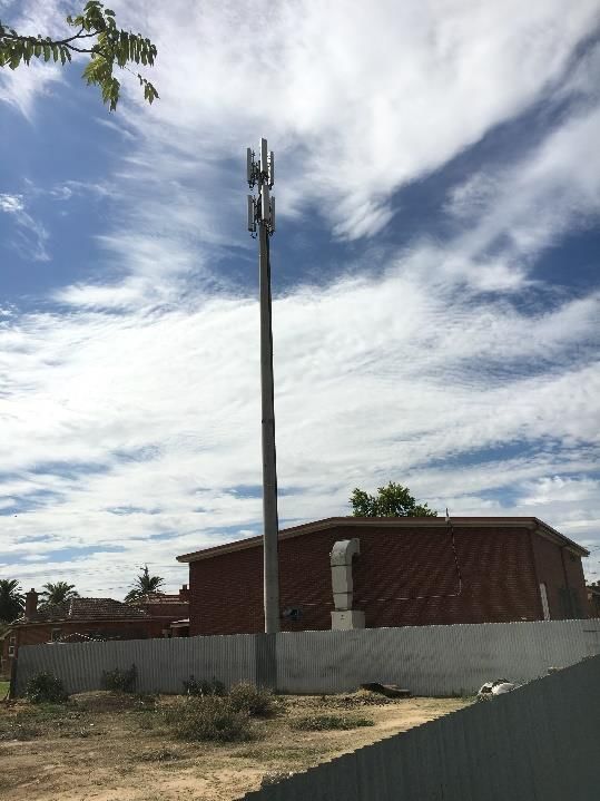
B.FLT.8009 – Getting Connected – Appendix 2

      Moving data and data speeds
Moving data (and associated information) around is based on two primary factors. The first is how
much data is needed to be conveyed, as measured in bits or bytes (we will focus on bits from hereon
in). This is, more or less, referring to the richness of the information conveyed. The second, which is
the one that ultimately affects our experience as movers of data (especially as consumers of data
and information) is how fast that data/information is conveyed. Here we are talking about data
transmission rates, which are considered in terms of bits per second (bps). To give an example of the
meaning of speeds, a typical voice call on a mobile phone would transmit the digital form of your
conversation to and from your handset at between 8 and 64 kbps (i.e. 8,000 - 64,000 bits per
second, here ‘k’ = kilo = 1,000). A digital TV streaming a movie from an internet site may deliver
upward of 83 kbps (lowest video quality) to as much as 833 kbps (i.e. 0.83 Mbps where 1 Mega =
1,000 kilo). At the other end of the scale are devices that periodically (i.e. not ‘live’ every second)
generate (and hence seek to move around) only small segments of data. A typical example is an
automatic weather station in a feedlot, which may seek deliver only a few kilobits of data (e.g.
temperature, humidity, wind speed) every 15 minutes or so.

The movement and consumption of data is a lot like using our cars; when you operate your car, you
can pay an initial premium for how fast it goes (i.e. at purchase), but when you are operating it, you
are not paying for how fast you drive it (unless you cop a speeding fine of course). Ultimately you
pay for the fuel that you pump into it. This is the accumulated effect of the speed/performance over
time. The same applies for data. You pay a component of a premium that is tied to how fast you
move data around, but principally, users pay for how much data (i.e. bits) is consumed, over a fixed
time period such as a month. This is the notion of data charges, which will be discussed later.

Different types of networks offer different transmission speed capabilities, which will be revealed as
we look closely at the sorts of connectivity options available.

2 Internal connectivity - Communicating with devices inside
  feedlots
The term ‘telemetry’ is used to define the automatic communications process whereby data are
collected at one location and transmitted to other locations for the purposes of monitoring. In the
context of feedlots today, we are talking about connecting devices internally within the feedlot
environment. There are a number of possible communications pathways to and from remotely
connectible devices. The pathways used are largely dictated by the volume of data that is to be
communicated, the speed at which it is to be transmitted, and also whether it is necessary to
transmit the data live or whether some form of latency is acceptable. This applies equally to whether
data is being sent to a remote device (for example for the purposes of actioning a command such as
releasing a gate or door latch in a shed, switching on heaters, lights or pumps and panning and
panning/zooming a remote camera), or whether data is being sent back from a device (such as a
weather station, remote camera, or a plethora of other plant, soil, water, environmental, animal or
asset sensors).

      Fibre connectivity

In terms of carrying capacity, that is data speeds, and a range of other technical considerations,
including immunity from electromagnetic interference (e.g. from electric fences and overhead
power lines) and lightning damage, the ultimate means of transporting data is the optical fibre.
Unlike electrical cables, namely copper wires, optical fibres convey data in the form of light pulses

                                                                                                Page 7 of 75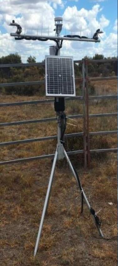
B.FLT.8009 – Getting Connected – Appendix 2

(‘1’ is on, ‘0’ is off). By using light pulses, it is possible to convey considerable amounts of data at
considerable speeds. Moreover, while all transmitted signals (optical and electrical) lose signal
strength with increasing transmission distance, optical fibres have better than an order of magnitude
lower attenuation rate with distance than copper. For example, over a distance of 100 m, an
electrical signal in a copper wire can fall as much as ~90% compared to an optical signal may
experience only a ~5% reduction in signal strength. It is for this reason that optical fibres constitute
the ground-based (terrestrial) backbone of telecommunications worldwide. Optical fibres are not
just used for external connectivity (e.g. for connecting homes via our national broadband network
and for connecting regions, countries and continents). Fibres can also be installed underground as
part of internal network connectivity, to form the future-proof (owing to the carrying capacity and
speeds) backbone of feedlots. Bearing in mind the current and emerging data needs of feedlots, and
in particular the focus on key operational locations within the feedlot such as the office, mill, pens,
induction sheds and hospitals, some feedlot operators are already installing fibre loops as the main
data haul conduits within their operations (Figure 2-1).

                                         (a)                                                             (b)

Figure 2-1. (a) An example schematic of a fibre loop installed in an Australian feedlot and (b) inside the feedlot office sits
a network service cabinet; the heart of an internal fibre loop within the feedlot precinct.

        Wired connectivity
The lowest cost solution, generally suited to distances up to 50 - 100 m, is via direct wire (co-axial)
cable connection. One advantage of this method is that you can also provide power via the same
cable and hence do not need solar panels at the power source. Cables can often be connected either
into a host computer (e.g. a serial port) or into the local area network (e.g. using a serial to ethernet
convertor).

                                                                                                                  Page 8 of 75
B.FLT.8009 – Getting Connected – Appendix 2

                    (a)                                                           (b)
Figure 2-2. An example of (a) an automatic weather station and (b) office vision from a weighbridge camera, both
connected directly into an adjacent feedlot office via cable.

Nowadays, this option is used in only the simplest (and shortest) of connections, for example, a
nearby weather station or weighbridge camera (Figure 2-2). The vast majority of devices and sensors
dispersed around a feedlot precinct are connected using entirely wireless means except, of course,
where linked through an internal feedlot fibre loop.

       On-farm radio networks – LANs, WLANs and WANs
When we refer to wireless telemetry, we are talking about radio networks. When the sensor output
is transmitted by a wireless transmitter, the assembly containing the sensor(s) and transmitter is
called a sensor ‘node’. The transmitting of data from one device to another within the farm
effectively constitutes an internal telecommunications network, which includes nodes and
communications links between them. While we are still talking about data and transmission speeds,
radio networks have a much broader lexicon of terms and physical concepts. The following
discussion clarifies some of the complexity around radio networks. The first step is to look deeper
into the basic elements of a network.

Networks can have different geometrical/spatial constructs and these are summarised in Figure 2-3.
A ‘node’ is where the sensor/device resides. Effectively, nodes are connection end-points and
multiple nodes may communicate with a ‘hub’, which can store information and forward it on to
other hubs (for example ‘store and forward’ systems). The information ultimately finds its way to the
point at which a connection is made to the outside world. The link to the outside world is known as
the ‘base station’ or ‘gateway’.

The nodes themselves can also play a direct role in the communication chain. Multiple nodes may
relay information between each other in a ‘mesh network’. Meshed network designs are becoming
more commonplace and sophisticated (Lamb, 2017 and references therein). ‘Self-healing’ mesh
networks are generating particular interest in the farming context for their ability to
transmit/receive information along alternative routes if one of the sensor nodes fail for some
reason. A star network, is a topology where nodes communicate individually, directly with a central
gateway. This topology is utilised in low powered wide area networks (LPWAN). At this point, a
discussion of network architecture is rather a theoretical exercise. The notions of node, hub and
base/station-gateways will be further illustrated when we discuss specific examples in later sections.

                                                                                                           Page 9 of 75
B.FLT.8009 – Getting Connected – Appendix 2

                                  (a)                                                          (b)

                                                            (c)

Figure 2-3. A basic network diagram as relates to (a) ‘store and forward’, (b) ‘mesh’, and (c) star farm sensor networks
(Extracted from Lamb, 2017).

There are a number of ‘classes’ of network based on the spatial scale. A local area network (LAN)
comprises fixed links/nodes within a limited area and is generally taken to be within buildings (like
the farmhouse), or a collection of buildings (e.g. shed precinct). A wireless local area network
(WLAN) is a wireless version of LAN using a wireless distribution method which gives users the ability
to move around within a local coverage area and yet still be connected to the network. A WLAN can
also provide a connection to the wider Internet. Most WLANs are based on the now ubiquitous ‘Wi-
Fi’ brand name. A wide area network (WAN) is a network that extends over a large geographical
distance. In the context of farms (including the farming land) we are talking about wireless WANs.
Often producers talk about Wi-Fi in their feedlots when talking about feedlot wide networks. Unless
they are talking only about in and around the office or other buildings/sheds ‘Wi-Fi’ (i.e. WLAN),
when it comes to longer range outdoor use, strictly speaking they are talking about a WAN enabled
by radio links utilising the frequencies also associated with their in-house Wi-Fi.

2.3.1 Radio transmission and antennas
The transmission range of wireless sensor nodes varies considerably. Radio range basically relies
upon three factors - frequency, power and environment. Some are designed for short-range, indoor
applications of a 50 – 100 m, while other sensors can transmit data to a receiver located tens of
kilometres away. As a general rule, the lower the frequency, which also means longer wavelength1,
then the better is the penetration characteristic and ability to refract (bend) around obstacles. Mind
you, the higher the frequency, the better the reflective properties of obstructions and this can
sometimes be used to advantage in reflecting a signal off an object rather than passing through it.
This is useful in back-scatter devices (which will be mentioned later). Generally, the lower the
frequency, the longer the transmission range; an assumption borne out of the fact that free space
(ie, open-air, line of sight) attenuation of radio waves increases with frequency. It is a little more
complicated because the way radio waves interact with obstacles is also dependent on the
frequency. Also, the frequency affects the performance of antennae; these are the devices at either
end of a link used to convert the electrical signals into radio waves and vice versa.

1
  Wavelength is always inversely related to frequency; i.e. higher wavelength means lower
frequency.

                                                                                                             Page 10 of 75
B.FLT.8009 – Getting Connected – Appendix 2
The frequencies at which we are allowed to transmit and receive radio signals across our landscapes
is governed by laws. Laws vary by country and region as to which parts of the wireless spectrum are
available for use without specific licenses. It stands to reason that those portions of the spectrum
that do not require licenses are more popular in terms of widespread commercial use. In Australia,
this includes 915 - 928 MHz and 2.4000 – 2.4835 GHz (Wi-Fi) (Australian Radiofrequency Spectrum
Plan 2013), and these are the major frequencies that manufacturers of farm radio devices tend to
use. As part of the industrial, scientific, and medical band (ISM), users do not need a radio license to
operate on these frequencies.
It is worth noting that there is no such thing as ‘unlicensed’ spectrum in Australia. Users must be
licensed to operate radiocommunication transmitters. However, the Australian Communications and
Media Authority (ACMA) management approach to the 915 MHz and 2.4 GHz bands is to apply a
'public park' concept with respect to devices considered ‘low-interference potential devices (LIPD)’.
Under the 'public park' concept, all LIPD users are able to access a small portion of the total resource
(the frequency band) and to share that resource in a way that requires minimal regulatory
intervention. Users of WLAN devices operating in these frequency bands are required to comply
with a set of conditions. The LIPD class stipulates no interference is to be caused to other
radiocommunications users, no protection from interference is offered and there is no licence fee
(ACMA 2016). An excellent discussion of currently available spectrum with respect to Internet of
Things (IoT) is given in IOTA (2016).
It is worth inserting a cautionary note here. Different countries/regions in the world have different
licence-free spectrum allocations and any user in Australia needs to be mindful of the fact that a
wireless transmitting device built in one country (for a domestic market) may not be compliant in
Australia (i.e. operates outside the allowed frequency bands or does not comply with the
requirements of the LIPD class) and hence would be illegal to operate without a specific licence.
For the purposes of introducing the basic principles and ultimately understanding how wireless
systems perform in Australia, we can now focus on two frequencies; ‘915 MHz’ and ‘2.4 GHz’ to
encapsulate the two most commonly used ISM ‘bands’. A relative measure of an antenna's ability to
direct or concentrate radio frequency energy in a particular direction or pattern is known as a ‘gain’.
The measurement is typically measured in dBi (Decibels relative to an isotropic radiator- or
antenna2). Antenna are divided into two basic classes - omni-directional and directional. Three
commonly used antenna designs are depicted in Figure 2-4.
2
An isotropic antenna is purely a theoretical construct; an antenna that can radiate uniformly in all
directions- i.e. out through a sphere. It is a useful benchmark in industry for comparing antenna
performance characteristics.
Page 11 of 75B.FLT.8009 – Getting Connected – Appendix 2
(a) (b) (c) (d)
Figure 2-4. Four common types of antenna (a) Omnidirectional (‘Omni’) and directional; (b) & (c) Parabolic grid or dish
(or semi-parabolic grid/dish) in two common forms and (d) Yagi (Source: (a) http://maxcomm.co.za; (b) http://www.l-
com.com; (c) www.ubiquiti.com and (d) https://www.scmsinc.com).
An omni-directional antenna (Figure 2-4a) radiates, or collects, radiofrequency energy from all
directions equally on a plane. The strength/sensitivity is highest at right angles to the length of the
antenna, decreasing to zero in a direction along the length of the antenna. The parabolic and Yagi
antennae (Figure 2-4b, c & d) are examples of directional antennae.
High ‘gain’ antennae are required to cover long distances. The gain of a reflector type antenna, such
as a parabolic grid or dish (Figure 2-4b, c) increases with increasing area of the parabolic surface, and
more so with higher frequencies. For example, for a given physical size, the antenna gain at 2.4 GHz
is significantly higher than an antenna at the lower frequency of 915 MHz. Alternatively, for a
required gain an antenna operating at the higher frequency can be physically smaller than that
operating at the lower frequency.
The deployment of an omni antenna versus directional antenna generally comes down to the
structure of the overall wireless sensor network (WSN) and the distances involved. A directional
antenna guides and receives energy from a predefined single direction. For example, a distant
sensor node would use a directional antenna to link with a base station/gateway. That base
station/gateway would similarly use a directional antenna if it was looking for just that sensor node
(Figure 2-5a). If the base station/gateway were receiving signals from multiple nodes in different
directions, then an omni antenna would be used on the base station/gateway (Figure 2-5b).
(a) (b)
Figure 2-5. A basic wireless sensor network (WSN) indicating use of different antenna types used in (a) point-to-point and
(b) point-to-multipoint links (Extracted from Lamb, 2017).
Page 12 of 75B.FLT.8009 – Getting Connected – Appendix 2
Atmospheric water vapour, fog and rain attenuate radio signals and the attenuation increases with
increasing frequency. Rain fade is the attenuation or interruption of wireless communications
signals resulting from water droplets (rain, mist, fog, snow) when the droplet separation is
comparable to the signal wavelength. Ultimately susceptibility to rain fade increases with increasing
frequency (shorter wavelengths), typically appreciable at higher frequencies, namely ≥11 GHz.
Both frequencies require "line-of-sight" for reliable operation. In many cases, the ability of an
obstruction to obstruct a signal boils down to its electrical conductivity (e.g. metal versus non-metal,
or water content) and its physical size. Physical size doesn’t mean how big the object is, rather its
similarity in size to the wavelength of the radio signal. For example, the higher frequency 2.4 GHz
signal has a shorter wavelength of 12.5 cm, whereas the lower frequency of 915 MHz signal has a
longer wavelength of 33 cm 3. Trees with leaves that have dimensions near the wavelength of 2.4
GHz, but which are typically shorter in length than the wavelength associated with of 915 MHz, will
cause higher attenuation at 2.4 GHz. Beyond this ‘rule of thumb’ it is difficult to quantify the
attenuation due to trees in the radio path.
For very long distance links, it is recommended that the antennas be elevated to clear all
obstructions. Here, we don’t just mean obstructions in front of the antenna, or in direct line of sight
between antennae. The entire radio beam from end to end looks like a long thin party balloon - thin
at the ends and thick in the middle. Attenuation kicks in if any part of that beam 4 ‘touches’ an
obstruction along the way. When transmission distances of 10 km or more are being considered, we
need to also factor in the curvature of the earth and atmospheric refraction (bending) in ensuring we
minimise ‘contact’. The 2.4 GHz has an advantage in this respect because, as it propagates through
the air from a directional antenna to its receiver, it swells out to a narrower radius than the lower
frequency 915 MHz waves. For example, at 2.4 GHz, for a 5 km link, the radius of the critical zone is
approximately 12 m at the midpoint (2.5 km). Note that over this modest distance, for ‘flat’ ground,
the curvature of the earth lifts the midpoint up another 0.5 m. That would require an antenna 12.5
m high at either end to avoid ‘contact’ with the ground. At 915 MHz the critical zone is
approximately 20 m in radius at the midpoint, plus that 0.5 m of extra ground height, meaning
antenna need to be 20.5 m high at each end. Put simply, the higher frequency of 2.4 GHz has the
advantage of requiring shorter antenna towers for any given ground, in addition to allowing for
smaller dimension (and lighter) antennae for any given gain requirements
2.3.2 Frequency, bandwidth, capacity and speed
The transmission frequency of a particular radio link refers to the ‘carrier’ frequency- that is the
frequency of the signal conduit that carries the information. The information to be transmitted is
coded onto the carrier waves; a process known as ‘modulation’. There are a number of ways of
coding the information onto the carrier, and a discussion of these can be highly technical. The
transmission (‘carrier’) frequency influences the amount of information that can be carried on the
signal and the way information is coded also affects the amount of information that can be carried.
Some of the basic terms often used in discussions of radio networks are defined and discussed
below.
There are two types of signal transmission- analogue and digital. Analogue transmission involves the
use of a continuous signal and is particularly suited to short range transmission (where repeaters are
not required), and in particular voice communications (e.g. CB/UHF radios). The information is
3
Wavelength is always inversely related to frequency; i.e. higher wavelength means lower
frequency.
4
Known as the first Fresnel zone
Page 13 of 75B.FLT.8009 – Getting Connected – Appendix 2
conveyed by modulating by one of two means; Amplitude Modulation (AM) and Frequency
Modulation (FM). Analogue transmission systems are increasingly becoming redundant to digital
transmission systems. Digital transmission involves the transfer of digital messages originating from
a sensor/transducer or from an analogue signal such as a phone call or a video signal, digitized into a
bit-stream using some form of analogue-to-digital (A/D) conversion and data compression method.
Digital Modulation is a generic name for modulation techniques that uses discrete signals to
modulate a carrier wave. The three main types of digital modulation are Frequency Shift Keying
(FSK), Phase Shift Keying (PSK) and Amplitude Shift Keying (ASK). IoT type devices and networks
involve almost exclusively digital communications.
Bandwidth is the difference between the upper and lower frequencies (in a continuous set of
frequencies) used to transmit signals; in other words the frequency range occupied by the coded
(modulated) carrier. For example, many radio channels have bandwidths of 20 MHz or 40 MHz. The
higher the carrier frequency, the higher the bandwidth. It is worth noting some basic definitions
here as they are sometimes used incorrectly. The signal bandwidth (as discussed before) is the range
of frequencies present in the signal, as constrained by the transmitter. The ‘Channel Bandwidth’ is
the range of signal bandwidths allowed by a communication channel without significant loss of
energy (attenuation). Probably the best way to appreciate the value of carrier frequency selection is
in terms of the following. The transmission of telephone-quality audio signal requires about 3 KHz of
bandwidth, while a TV quality transmission requires about 4 KHz; and there are approximately 10
times more of these bands between 2 and 3 GHz than there is between 900 MHz and 1 GHz.
Applying the same logic, the higher frequency of 2.4 GHz has higher available bandwidth compared
to the lower 915 MHz frequency.
Finally, the Channel Capacity or Maximum Data rate (or bit rate) is the ‘transmission speed’
introduced earlier. This is, again, the maximum rate (in bits per second - bps) at which data can be
transmitted over a given communication link, or channel. It therefore stands to reason that the
higher the carrier frequency, the higher the upper limit of the modulation frequency available to
encode information on that carrier. Signal strength is a key variable in transmission speed of any
radio device. Assuming there is no network-imposed constraints at either end of wireless
transmission link, speeds increase in proportion to signal strength (or bandwidth). In the absence of
any obstruction effects, halving the distance to an omni-directional antenna increases the signal
strength by 22 = 4 times. This is the so-called ‘inverse-square law’. A reality of transmission networks,
however, is that systems at either end will invariably constrain speed for any given signal strength
between the transmitter and receiver.
With ever increasing numbers of radio sources/receivers, interference and security are key
considerations. Rather than a single carrier frequency, a transmitter can broadcast the information
using a range of frequencies; known as ‘spread spectrum’. ‘Frequency hopping’ (FHSS) involves
rapidly switching the carrier wave amongst numerous frequency channels, using a ‘pseudorandom’
sequence known to both the transmitter and receiver. Another method, direct-sequence spread
spectrum (DSSS) involves adding known noise to the transmitted signal. The popular Wi-Fi uses a set
of pre-defined frequencies (channels) within its allocated portion of the 2.4 GHz spectrum.
Frequency, or ‘Channel hopping’ is one means of avoiding interference between multiple Wi-Fi
networks, for example in a feedlot environment.
Spectral efficiency, spectrum efficiency or bandwidth efficiency refers to the data rate that can be
transmitted over a given bandwidth. Measured in bits per second per unit frequency slice (i.e. per
Hz; namely bps/Hz), spectral efficiency is a measure of how efficiently a limited frequency spectrum
is utilized by the communications system and is, for example a measure of the quantity of users or
services that can be simultaneously supported by a limited radio frequency bandwidth in a defined
Page 14 of 75B.FLT.8009 – Getting Connected – Appendix 2
geographic area. It may be defined as the maximum aggregated throughput or ‘goodput’, summed
over all users in the system, divided by the channel bandwidth. This measure is affected not only by
the single user transmission technique, but also by multiple access schemes and radio resource
management techniques utilized. Typical Wi-Fi spectral efficiencies (per site) range from 0.9 to 1.2
bps/Hz.
2.3.3 Transmission power
In addition to the physical design of antennae, transmission power is a key factor in determining the
range of wireless systems (and data speeds). The power of a transmitter (or the signal strength
experienced by a receiver) is measured in dBm, which is the decibel scale referenced to 1 milliwatt (1
mW). A power level of 0 dBm corresponds to a power of 1 mW. As the decibel scale is a logarithmic
scale, a 10 dB increase in level (+10 dB) is the same as a 10x increase in power- likewise -10dB
equates to 1/10th of the power, or in this case 0.1 mW.
The power level of a transmitter is defined in terms of, again, a hypothetical isotropic radiator
(antenna). In radio communication systems, the equivalent isotropically radiated power (EIRP) is the
amount of power that a theoretical isotropic antenna (which evenly distributes power in all
directions) would emit to produce the peak power density observed in a given direction from the
deployed antenna. When installing a wireless system with an external antenna, the EIRP calculation
of the assembled device should not exceed the Australian class license limit. For example, the LIPD
class which is where the majority of connected devices would seek to operate. Ultimately when
installing a system, the user either adjusts the transmitter power output, the length of cable
between the transmitter and the antenna (which itself introduces attenuation) and/or the choice of
antenna (gain).
Power levels are capped (ACMA 2016). As with frequency selection, care must be taken to ensure
any purchased equipment, especially from overseas that may be destined for a domestic rather than
export market, complies with power caps. Australian regulations allow higher overall output power if
the system uses spread-spectrum techniques (ACMA, 2016). Higher field strengths are allowed
because spread-spectrum systems are:
less likely to interfere with other systems compared to single-frequency transmitters,
more immune to interference from (or causing interference to) other systems, and
utilise the available bandwidth more efficiency.
For example, devices operating under the LIPD class licence in the 915 – 928 MHz range are limited
to 1W EIRP whereas a maximum radiated power of 4W EIRP is authorised in the 2.4 – 2.4835 GHz
band for digital modulation transmitters or for frequency hopping transmitters that use a minimum
of 75 hopping frequencies (ACMA, 2016b).
In summary, over long-distance links, several factors contribute to the radio link performance. It is
not the purpose of this review to recommend designs. Even though the open-air (free- space) loss at
915 MHz is lower than at 2.4 GHz for purely physics reason, when you consider the typical antenna
gains and antenna heights required to clear obstructions, a 2.4 GHz radio link often has the
advantage.
Users of the two key frequency bands and in particular the 2.4 GHZ band, are experiencing
increasing levels of interference because so many devices around us use the same band. The
unregulated ‘public park’ concept applied to this band renders responsibility of managing
interference on the user. The extension of wireless WANs over longer ranges, and the concentration
Page 15 of 75B.FLT.8009 – Getting Connected – Appendix 2
of multiple separate systems on common infrastructure, such as local towers, often brings the
challenge of interference to a head. There are community wireless groups that work to grow
awareness of such issues and promote open communications between networks to mitigate the
effects of interference when designing and deploying WANs. One example, Air-Stream Wireless Inc.
(ABN 63553275830; Walkerville SA) is committed to “minimizing the impact of interference through
public awareness and providing an open platform for wireless LAN users to share information to
maximize the effectiveness of their equipment and minimizing interference” (Air-stream Wireless,
2016).
Given the undeniable (and unavoidable) physics at play, the regulatory environment within which all
producers and technology providers have to work and the increasingly congested airspace within
which we are all trying to co-exist, there is one certainty all producers must face in deploying WSNs
on their farms. The transmit/receive performance of any WSN will never be as it is ‘on the box’.
Without a doubt, the first step for any producer wishing to deploy or modify a WSN on their farm is
to undertake a radio strength test across the farm landscape to ascertain the best locations for those
transmitters and receivers.
2.3.4 Store and forward telemetry
Store and forward telemetry systems are useful where large distances are involved. Intermediary
hubs act as repeaters (Figure 2-3a). Numerous innovative systems have been designed with the
capability to receive and store information, and then retransmit them onwards as available
bandwidth allows. As the name suggests, these systems retain data at the hubs until successfully
passed on to the next hub or gateway which is good for data security. Typical examples, such as the
2.4 GHz Dosec Design/ICT International system (Figure 2-6) will store data at the nodes and hubs
whenever the communications channels fail or during congested transmit/receive periods, and
synchronously forward packets whenever the channel is open. The data packets ultimately end up at
the network gateway.
(a) (b)
Figure 2-6 (a) Example of a 2.4 GHz store and forward telemetry system developed by Australian companies ICT
International (www.ictinternational.com) and Dosec Design (www.dosec.com.au). Note the omnidirectional antenna on
the top of the tower for receiving signals from nearby nodes and the directional antenna beneath it for forwarding the
signal to the next node/gateway. (b) Web server user interface providing updated signal strength and hub/node health
information (nodes = blue icons, hubs = green icons) (Extracted from Lamb, 2017)
Page 16 of 75B.FLT.8009 – Getting Connected – Appendix 2
2.3.5 Mesh networks
Like the other network architectures, mesh networks are finding increasing use on farms. The use of
the ZigBee radio standard (IEEE 802.15.4) which facilitates a ‘self-healing’ capability is particularly
desirable given the harsh environmental conditions in which many sensor nodes have to exist (e.g.
cattle grazing, weather). ZigBee radios allow the network to actively change pathways to suit
conditions. Moreover, typical mesh sensor networks have the added capability to hold data for an
end or router node while waiting for it to ‘wake up’. This offers a level of data security but also
supports the use of devices that can be allowed to ‘sleep’ when not being used to collect
measurements, and hence save battery power.
Given that each ‘hop’ in communicating data from a given sensor to the gateway (Figure 2-3b)
penalises the bandwidth/speed, mesh networks are particularly suited to relatively small-scale
deployments on farms, or where node density supports low signal strength transmissions, small bit
messages and the landscape provides for high node visibility (Figure 2-7). One example is Australian
company AirMesh (www.airmeshelectronics.com.au) which utilises Modbus, a serial communication
protocol over ZigBee.
Whilst not related to deployed ‘things’ directly, the use of mesh network technology is also being
trialled for providing internet access to users who would otherwise not have it, by creating
intelligent community networks bridging to those locations that do have it. One example is WYSPS
(www.wysps.net.au), which is undergoing some limited trial work in Bega, NSW (Eckelmann, 2017).
While in its infancy, the use of low cost Wi-Fi nodes (~$20) (Figure 2-8) is desirable, but with ‘hop’
ranges of only up to 50 m, multiple hops are required to reach the neighbour’s boundaries which
subsequently penalises bandwidth/speed to that neighbour. Moreover, it has been found to be
difficult to find neighbours willing to share their bandwidth into the mesh community when their
own bandwidth (e.g. ADSL2 or wireless NBN) is already being fully utilised at home.
Page 17 of 75B.FLT.8009 – Getting Connected – Appendix 2
(a)
(b) (c)
Figure 2-7 (a) 3 nodes (circled) of a (b) 100-node self-healing mesh network and user interface, (c) mesh gateway receiver
and mobile network modem (Extracted from Lamb, 2017).
Figure 2-8. An example of a low-cost Wi-Fi node capable of forwarding internet access as deployed in a community
WYSPS mesh network (Extracted from Lamb, 2017).
Page 18 of 75B.FLT.8009 – Getting Connected – Appendix 2
2.3.6 Long range/lower power WAN– 915 MHz
While limited in bandwidth compared to 2.4 GHz, a significant focus area of on-farm network
technology and for data/information service providers is long range and/or lower power radio
devices (LoRaWAN/LPWAN) utilizing the 915 MHz band. LPWAN technologies are designed for
machine-to-machine (M2M) and IoT networking environments. With decreased power
requirements, longer range and lower cost than a mobile or 2.4 GHz network, LPWANs are
considered by many to enable a much wider range of M2M and IoT applications which, to date, have
been constrained by budgets and power issues. Importantly, LPWAN data transfer rates are very
low, often less than 5 kbps and only 20-256 bytes per message are sent several times a day.
Consequently, the power consumption of connected devices is very low, often supporting battery
life in the range of years; up to 10 years in some cases. LPWAN enables connectivity for networks of
devices that require only low bandwidth and typically utilises a ‘star’ topology (Figure 2-3c). The
networks can also support more devices over a larger coverage area than consumer mobile
technologies and have better bi-directionality. While Bluetooth, ZigBee and Wi-Fi are generally
favoured for consumer-level IoT implementations, the need for a technology such as LPWAN is much
greater in agriculture where:
distance is a major consideration,
sensor numbers will likely be high,
power consumption needs to be low, and
only small packets of information, such as from soil moisture probes, device sensors (e.g.
pumps, gates and weather stations) are required (Figure 2-9).
Taggle (www.taggle.com.au) is an example of a LPWAN system. Operating in the 915 MHz LIPD band,
these transmitters are designed to send small packets of information (for example water meters and
weather station data) over long distances, typically up to 5 km, but observed up to 50 km in rural
environments.
(a) (b) (c)
Figure 2-9. (a) A water tank sensor and transmitter, (b) close-up of low power transmitter and (c) Taggle LR/LP base
station receiver (vertical aerial) and mobile network gateway (small white ‘bulb’ antenna located on protection cage)
(Extracted from Lamb, 2017).
Page 19 of 75B.FLT.8009 – Getting Connected – Appendix 2
2.3.7 LORA-WAN
LoRaWAN is a particular LPWAN specification intended for battery-powered devices that support
low-cost, mobile, long range and secure bi-directional communication for IoT and M2M (LORA
Alliance 2017; The Things Network 2017). The LoRaWAN protocols are defined by the LoRa Alliance
and formalized in the LoRaWAN Specification. The LoRA Alliance is an open, non-profit association
initiated by industry leaders to standardize LPWAN being deployed around the world. LoRaWAN is
designed to allow low-powered devices to communicate with Internet-connected applications over
long range wireless connections. Devices operate in the LIPD class spectrum, namely 915 – 928 MHz
band, and are optimized for low power consumption and is designed to support large networks with
considerable numbers of devices. LoRaWAN features include support for redundant operation,
geolocation, low-cost, and low-power. A LoRaWAN Specification document describes the
LoRaWAN™ network protocol (LORA Alliance 2017).
A key desirable aspect of LoRaWAN devices, as it relates to agriculture (and other industries) is the
commitment to a set of standard specifications, allowing developers of sensors to provide
immediately compatible, fit-for-purpose devices on farm. At the other end, service providers can
develop web-based information delivery systems or utilize bespoke cloud-based solutions. The
Things Network (The Things Network, 2017) is a global initiative, an open network, that provides
resources and supports developer forums, virtual labs and communities
(www.thethingsnetwork.org/labs).
Companies in Australia such as Meshed (www.meshed.com.au) consider themselves as technical and
service facilitators of connected technologies, and focus on the provision of development kits and
bespoke gateways, allowing developers to focus on sensor innovations and the development of
decision support and information delivery systems at the other end. Thinxtra (www.thinxtra.com)
offers additional connectivity and cloud capacity through partner SigFox (www.sigfox.com). Both
offer developer kits suited to Australian conditions (including spectrum) (Figure 2-10 a, b). Thinxtra
partners with developers around the world to develop solutions (Figure 2-10 c, d). Example devices
include irrigation flow sensors, soil sensors and wearable livestock monitoring devices.
Page 20 of 75B.FLT.8009 – Getting Connected – Appendix 2
(a) (b)
(c) (d)
(e) (f)
Figure 2-10. IoT device development kits relevant to feedlots (a) Meshed ‘Multitech mDot Micro Developer/Programmer
Kit’ (Source: http://meshed.com.au/product/multitech-mdot-micro-developer-kit/), and (b) Thinxstra ‘Sigfox Pi’ designed
to support Rasberry Pi devices (Source: http://www.thinxtra.com/devicemakers-dev-kits/). Examples of relevant third
party-developed devices; (c) wearable animal devices from Spanish company Digit Animal, (d) remote worker sensor
Thixtra Xpress (Source: https://www.thinxtra.com/portfolio-item/lone-worker-monitoring/), (e) Silo level sensor developed
by French partner GreenCitizen (Source: http://www.greencityzen.fr/en/produits-en/hummbox-level-connected-ultrasonic-
level-sensor/) and (f) Tank or storage level sensor. All examples are fully compatible with the SigFox data management
system.
Page 21 of 75B.FLT.8009 – Getting Connected – Appendix 2
2.3.8 Point-to-point links within feedlots
Point-to-point links between feedlot offices and key operations locations such as induction sheds,
yard/pens and mills is an important wireless connectivity option for managers wishing to run key
software platforms including Digi-Star and Elynx platforms (discussed below) on location where the
platform is located on servers either in the nearby feedlot office or (via an external connection point
on the feedlot, for example the office) on a server located at headquarters in another
region/location entirely. Such internal point-to-point links utilise directional antenna and rely upon
Wi-Fi frequencies (2.4 GHz) or, in some cases the higher frequency (hence higher bandwidth) Wi-Fi-
‘n’ frequency (5 GHz) (Figure 2-11).
(a) (b)
Figure 2-11. Examples of a point to point link between (a) an induction shed and (b) feedlot office. The induction shed has
a parabolic dish and the feedlot office uses a Yagi to facilitate the link.
Typical speeds between a wireless router (for example located in the Office where external
connectivity is linked) and client devices at the end of a Wi-Fi link depends very much on the nature
of the link technology. The physical layer (PHY) rate is the maximum speed that data can move
across a wireless link between a wireless client and a wireless router. User activities like file transfer
and web content browsing happen at the application layer. The rate obtained at the application
layer will be much lower than the physical layer rate. For example, a typical link rate of 300 Mbps
usually corresponds to 50 to 90 Mbps speed on applications layer. In other words, this is the
realisable speed (from a user perspective) through the link.
Examples of the platforms that rely on point-to-point links include Elynx and Digi-Star platforms.
Elynx is a software and information technology service providing a suite of products including:
StockaID (individual animal identification and management software program design to
record numerous parameters via readers or manual input),
FY 3000 (a suite of projects including Feedlot 3000, which is an integrated management
system that imports data from the StockaID program and exports financial data to financial
accounting software programs), and
Bunk Management System (a simple commodity and feedbunk management system to
manage animal movements on a lot or pen basis).
Page 22 of 75B.FLT.8009 – Getting Connected – Appendix 2
Digi-Star is a brand of weight management software to manage feed mixes. It includes Beef Tracker,
which is a Windows ® based feed management software system that works in conjunction with the
scales on a feed mixer truck and allows management and collection of feed batching and delivery
weight data.
3 External connectivity
Telecommunications Networks
As with any other subscriber, feedlots will access one or both of two types of telecommunications
networks; fixed and/or mobile. This relates to the level of mobility afforded to subscribers. A fixed
network is where a call/data exchange is initiated or received at the subscriber’s premises, such as
the office. In a mobile network, a call or data can be initiated or received by an individual handset at
any place in which the network operates. Some feedlot offices, while obviously at a fixed location,
may access the network via a mobile network (for example using a mobile booster antenna on the
office roof - discussed later), which is then accessed via desk-top phones (giving all the appearance
of a landline though it is actually utilising the mobile network).
In its simplest form (Figure 3-1), fixed networks consist of multiple local access networks, linked
together by a transmission ‘backhaul’ network. The local access network includes the connection
between each subscriber and a local network node, commonly known as an exchange or switching
point, by way of particular transmission media, such as copper wire, optical fibre, mobile, wireless or
satellite technology. Normally, the network also includes a further transmission link from this node
to a major network node that aggregates and interconnects traffic from a number of exchange or
switching points. This is a general hierarchy, although it should be noted that the exact hierarchy of a
telecommunications networks varies with operators.
‘Backhaul’ is a word commonly encountered in telecommunications discussion. Backhaul refers to
the medium and long distance optical fibre and microwave transmission networks that connect local
exchanges, main exchanges and mobile and fixed wireless towers between all population centres in
Australia (Figure 3-2). Backhaul networks carry voice and data transmissions. In everyday language,
backhaul, which is essentially the wholesale transmission market, is generally associated with the
commercial entities that provide and manage it. For example, NBN Co, Telstra and Optus operate
substantial backhaul transmission networks.
Providers of backhaul guarantee a quality of service (QoS) to other carriers that utilise their
networks as well as retailers of the service to subscribers. Quality of service refers to the
performance of the network, in particular as experienced by users of the network (Lamb, 2017)
Typically, users specify performance requirements and the network commits its bandwidth making
use of different QoS schemes to satisfy the request. QoS can be degraded by congestion, which is
caused by traffic overflow (bottlenecks); delays, caused by sub-optimal performance of networking
equipment under large loads, as well as caused by distance or retransmission of lost packets; shared
communication channels, where collision and large delays become common; and limited bandwidth
networks with poor capacity management. This is often confused by quality of experience (QoE),
which focusses on user perception of quality. Generally, assessments of telecommunications
performance, and, in particular, as it relates to broadband, is given to mean data transfer rate (e.g.
internet access speed) (ACCC 2016a).
Page 23 of 75You can also read