GNSS total variometric approach: first demonstration of a tool for real time tsunami genesis estimation - Nature
←
→
Page content transcription
If your browser does not render page correctly, please read the page content below
www.nature.com/scientificreports
OPEN GNSS total variometric approach:
first demonstration of a tool
for real‑time tsunami genesis
estimation
Michela Ravanelli 1*, Giovanni Occhipinti2,3, Giorgio Savastano4,5, Attila Komjathy4,
Esayas B. Shume4,6 & Mattia Crespi1
Global Navigation Satellite System (GNSS) is used in seismology to study the ground displacements
as well as to monitor the ionospheric total electron content (TEC) perturbations following seismic
events. The aim of this work is to combine these two observations in one real-time method based on
the Total Variometric Approach (TVA) to include the GNSS real-time data stream in future warning
systems and tsunami genesis estimation observing both, ground motion and TEC. Our TVA couples
together the Variometric Approach for Displacement Analysis Stand-alone Engine (VADASE) with the
Variometric Approach for Real-Time Ionosphere Observation (VARION) algorithms. We apply the TVA
to the Mw 8.3 Illapel earthquake, that occurred in Chile on September 16, 2015, and we demonstrate
the coherence of the earthquake ground shaking and the TEC perturbation by using the same GNSS
data stream in a real-time scenario. Nominally, we also highlight a stronger kinetic energy released in
the north of the epicenter and visible in both, the ground motion and the TEC perturbation detect at
30 s and around 9.5 min after the rupture respectively. The high spatial resolution of ionospheric TEC
measurement seems to match with the extent of the seismic source. The GNSS data stream by TVA of
both the ground and ionospheric measurement opens today new perspectives to real-time warning
systems for tsunami genesis estimation.
Natural hazards such as earthquakes and the subsequent tsunamis generate atmospheric acoustic-gravity waves
that propagate upward to the ionosphere where they may be detectable by ionospheric sounding techniques1. In
particular, at the epicentral area, the uplift at the surface—produced by the seismic rupture—induces, by dynamic
coupling with the atmosphere, an acoustic-gravity wave (AGWepi ). During the upward propagation the AGWepi
is strongly amplified by the double effects of the decrease of the air density ρ and the conservation of the kinetic
energy ρv 2, under the adiabatic hypothesis of the atmosphere. Consequently the oscillation v induced by the
crossing of the AGWepi is becoming large enough to generate strong perturbations in the ionospheric plasma,
mainly where its density is near the maximum (F-layer, altitude about 300 km)2.
Different techniques have been already applied to detect the ionospheric post-seismic perturbations:
ionosondes3, HF Doppler s ounders4,5, airglow c ameras1,6–8, over-the-horizon r adar8,9 and GNSS sTEC (slant
TEC, TEC on the satellite-receiver line-of-sight LoS) o bservations10–14. This last technique received more and
more attention due to the wide and continuously increasing worldwide availability of GNSS permanent stations.
GNSS sTEC became a major tool to study the i onosphere15, which can be affected by geophysical events such as
earthquake1,2,16, tsunami17–20, volcano e xplosions21–23; and man-made events such as e xplosions24,25 and rocket
launches26–28. Recently, an algorithm was d eveloped29,30, named VARION (Variometric Approach for Real-Time
Ionosphere Observation), able to estimate sTEC variations from GNSS observations in real time. GNSS-sTEC
measurements are commonly referred to the altitude of the F-layer along the LoS, called the ionospheric piercing
point (IPP). The AGWepi for large events (Mw > 7) is systematically detectable near the e picenter2, within 1000
km, and they move vertically at the speed of sound c s . In the Earth atmosphere c s varies with the altitude (from
several hundreds m/s—near sea level—to about 1 km/s at 400 km of altitude); c s ranges from 800 to 1000 m/s
1
Sapienza University of Rome, via Eudossiana 18, Rome 00184, Italy. 2Université de Paris, Institut de Physique
du Globe de Paris, CNRS, 75005 Paris, France. 3Institut Universitaire de France, Paris, France. 4Jet Propulsion
Laboratory, 4800 Oak Grove Dr, Pasadena, CA 91109, USA. 5Present address: Spire Global, Inc., 33 Rue
Sainte‑Zithe, 2763 Luxembourg, Luxembourg. 6Present address: California Institute of Technology, 1200 E
California Blvd, Pasadena, CA 91125, USA. *email: michela.ravanelli@uniroma1.it
Scientific Reports | (2021) 11:3114 | https://doi.org/10.1038/s41598-021-82532-6 1
Vol.:(0123456789)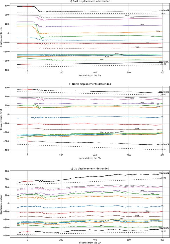
www.nature.com/scientificreports/
at the height of the ionospheric F-layer ( 300 km), where the electron density reaches the maximum11. Overall,
it takes around 8 min for the AGWepi to be detectable by GNSS-sTEC observations.
The recent work of Manta et al.16 clearly shows the empirical relationship between the TEC perturbations and
the maximum volume of the displaced water during the tsunami genesis (source extent times the max uplift at
the source). Authors highlighted the potential use of GNSS-sTEC observations for tsunami genesis estimation
at 8 min after the rupture to support conventional tsunami warning systems. They introduced the ionospheric
tsunami power index (ITPI) empirically related to the maximum volume of displaced water (in km3) during the
tsunami genesis to discriminate tsunamigenic earthquakes.
On the other hand, it has been known and tested that earthquakes induced ground shaking and coseismic
displacements that can be effectively recorded using GNSS as w ell31–36. The ground motion measured by GNSS
is benefiting of its relevant feature not to be affected by the saturation problem, which can impact seismometers
located near the epicenters of strong earthquakes. A great effort in the last decade has been done in order to
explore the contribution of GNSS data in the future tsunami warning systems in order to improve their reliabil-
ity of the responses. Ground motion measured by GNSS receivers has been used to estimate the magnitude37,
moment tensor38 as well as finite s ource39, in particular for tsunamigenic events and to improve the tsunami
genesis estimation40. Also in this case, the real-time approach, named VADASE (Variometric Approach for
Displacements Analysis Stand-Alond Engine), was proposed by Colosimo et al.41 and refined in Fratarcangeli et
al.42 to estimate seismic waveforms and coseismic displacements.
We introduce here the dual GNSS real-time contribution using the same data-stream from permanent stations
for both ground shaking and TEC estimation, to explore the potential improvement of tsunami genesis estima-
tion. We coupled the VADASE and VARION algorithms—the former being able to estimate surface waveforms
and co seismic displacements41,42, and the latter is able to compute sTEC perturbations in real-time29,30.
The final algorithm, named Total Variometric Approach (TVA), was applied to the moderate tsunamigenic
earthquake of Illapel (Chile, September 16, 2015, Mw 8.3). We analyse the GNSS permanent stations already
providing real-time data stream; as well as the GNSS stations (not real-time) but used here in a real-time scenario
to improve the coverage of our network. We also support the GNSS ground motion observations with traditional
accelerometer measurements.
In particular, we first introduce the Illapel event and the response of tsunami warning systems; then we detail
the dataset and the methodology used in the investigation; and we finally present our results and conclusions.
Earthquake information and dataset
The 2015 Illapel earthquake, in Chile, occurred 46 km offshore of the Coquimbo region on September 16 at
19:54:33 Chile Standard Time (22:54:33 UTC), with a moment magnitude of Mw 8.3. The initial quake lasted
between 3 and 5 min and it was followed by several aftershocks greater than moment magnitude 6.0, and two
of them exceeded 7.043. The earthquake occurred on thrust faults along the boundary of the Nazca and South
American plates. The region frequently produces large earthquakes that induce deadly tsunamis.
A tsunami threat message from NOAA Pacific Tsunami Warning Center was issued 7 min after the main
shock44,45 and Servicio Hidrográfico y Oceanográfico de la Armada (the organization in charge of the Chile’s
National Tsunami Warning System) issued the first tsunami alarm 8 m in46 after the earthquake: despite the
47
prompt evacuation, eight causalities were attributed to the t sunami . The first tsunami waves arrived on the
Chilean coast within 10 min48, with a series of waves reaching at least 4.5 m49 on the closer coasts and produced
severe damages and losses.
Different datasets were employed for VADASE and VARION algorithm. Nominally, 44 GPS stations at 1 Hz
rate from Centro Sismológico Nacional, Universidad de Chile were employed for VADASE algorithm: the dataset
is shown in the right panel of Fig. 1. The high-rate data (1 Hz or more) are required to avoid aliasing in the
estimation of ground shaking and waveforms.
Data from 118 GPS stations, mostly located in Chile but also spread all over the South-American conti-
nent, were processed with VARION, as it is shown in Fig. 1 (left panel). Nominally, 48 GPS stations (including
the previous 44, since they also supply data at 15 s rate), located in Chile were kindly provided by the Centro
Sismológico Nacional, Universidad de Chile (CSN). Other observations were gathered from 15 GPS stations of
International GNSS service (IGS), from 26 GPS stations of Système d’Observation du Niveau des Eaux Littorales
(SONEL) network and from 29 GPS stations of Low-Latitude Ionospheric Sensor Network (LISN) respectively.
These GPS receivers collected data at 10, 15 and 30 s rate.
It is important to underline that only 21 stations of 118 stations can already work in real time. For real time,
we mean the possibility for a GNSS receiver to broadcast real-time streaming of GNSS/GPS (RT-GNSS) data in
RTCM formats50 via the Networked Transport of RTCM via Internet Protocol (NTRIP)51. In detail, the GPS sta-
tions belonging to CSN are not all able to provide data in real time at this point. Both IGS and SONEL networks
include GNSS receivers from national and regional networks: few of them are technically set up to provide data
in real time . Nevertheless, the 29 stations from LISN can provide GNSS measurements in near real time (every
15 min). Therefore, it is important to push forward enhancing the GNSS network in a real-time operational
approach.
Ground shaking and coseismic displacements from VADASE
GNSS high-rate observations (1 Hz) were used as input for the VADASE algorithm to estimate the east-, north—
and up-components of the velocity for each receiver. The upper panel of Fig. 2 show the up-component of veloc-
ity: the series are sorted according to GNSS receiver distances (computed with Vincenty’s f ormula52) from the
epicenter. Positive and negative distances represent respectively the GNSS stations placed north and south of
the epicenter. Velocity time series for the horizontal and the up-components for CMBA station (the closest one
Scientific Reports | (2021) 11:3114 | https://doi.org/10.1038/s41598-021-82532-6 2
Vol:.(1234567890)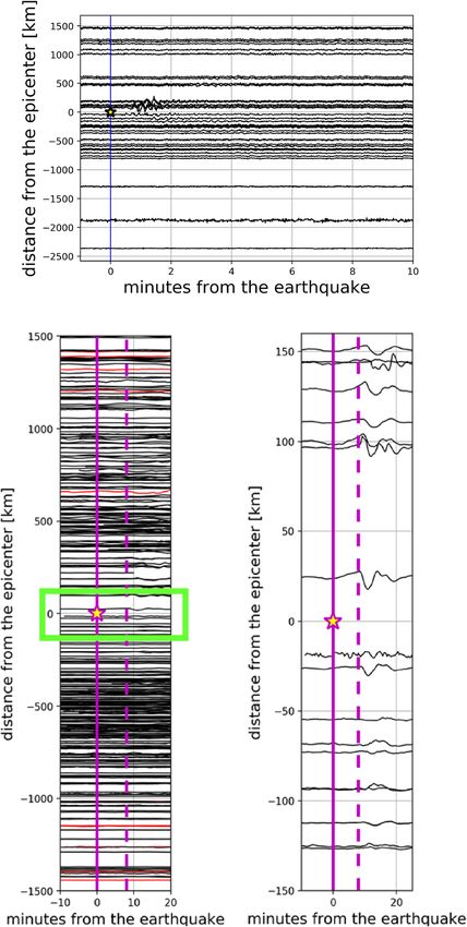
www.nature.com/scientificreports/
Figure 1. Left—Map with the epicenter of the earthquake and the 118 GPS permanent stations at low-rate
data sampling (10, 15, 30 s) used in VARION processing for sTEC variation estimation; GPS stations from
CSN, SONEL, IGS and LISN in red, blue, orange and green respectively. Right—Map with the epicenter of the
earthquake and the 44 GPS permanent stations at high-rate data sampling (1 s) used in VADASE processing for
ground shaking and kinetic energy estimation: CSN stations in blue.
to the epicenter towards North) are shown in Fig. 3a,b. The earthquake significant shaking was detected on the
basis of the Levene test for equality of variances at around 30 s after the rupture. The moving window was 60
samples, corresponding to 1-min interval, and the significance level for the test was equal to 1%.
The interval corresponding to the earthquake significant shaking represents is selected between 100 and 200
s after the earthquake (highlighted in red in Fig. 3a,b). Nominally, Fig. 3a shows the horizontal component of
the velocity for the GNSS stations CMBA, in essence the shaking of the receiver in the horizontal plane. It is
important to recall that the shaking duration through Levene test was evaluated on the lesser noisy horizontal
component of the velocity (east- and north-components combined), and then the same interval was considered
for the up-component.
The determination of the shaking duration allows to estimate the coseismic displacements and the energy
released (see Methods section for computation details) by the earthquake for every GNSS receiver. Left panel of
Fig. 4 shows the kinetic energy associated to the Up component for each GNSS station: the size of each station
is proportional to the kinetic energy. The kinetic energy (Table 1) released northbound is remarkably higher
than the southbound one.
The same procedure was also applied to accelerometer data showing similar results: accelerometers located
north are characterized by larger ground shaking than south. In Supplementary Material (SM) we show the
accelerometer network (Fig. SM1), the different step to the energy determination for one single accelerometer
(Fig. SM2) and the map of released energy by accelerometers (Fig. SM3).
In order to visualize the time evolution of the ground displacement, Fig. 5 shows the coseismic de-trended
displacements series as computed by integrating the VADASE velocity solutions, the trend is also showed on the
same figure (Fig. SM4 shows coseismic displacements before the de-trending operation). Table 1 summarizes
the overall coseismic displacements. The largest coseismic displacement occurs for the east-component and this
is consistent with the east-northeast movement of the Nazca p late43. Moreover, the greatest east displacements
take place for the stations placed at north of the epicenter.
We used the shaking duration to determine the energy released by the earthquake in 100–200 s after the
earthquake. The Power Spectral Density (PSD) related to this duration was computed from the Up component
of the velocities. In Fig. 3c, the PSD respectively for CMBA stations is reported. The normalized kinetic energy
associated to the vertical shaking has been calculated by integrating the PSD within the frequency range 3.3-200
mHz. This frequency range was chosen in order to include the acoustic component of the typical AGWepi , and
this is highlighted in Fig. 3c ; the upper limit of 200 mHz was chosen after a trial and error procedure in order
to catch the whole normalized kinetic energy asymmetry. Figure 3d depicts the energy spectrum for CMBA
station for the up velocity component.
Ionospheric detection of the AGWepi by VARION
In order to exclude other sources of ionospheric disturbances (e.g., geomagnetic storms), we evaluate relevant
geomagnetic indices53 during the day of the earthquake. The official planetary K p index does not reach the value
of 4, excluding the possibility of geomagnetic storms on that d ay54. DST index (Disturbance Storm Time) was
about—19 nT before and after the earthquake t ime53. Hence, according to Loewe and Prölss55 classification, it
is possible to state that no geomagnetic storm was present on that day and so the Illapel earthquake is the main
source of the ionospheric perturbations.
In order to perform the localization of the TEC perturbation detected by the GNSS stations in real-time, we
compute the ionospheric piercing points (IPPs) fixing the layer of the ionosphere at the maximum of ionization
Scientific Reports | (2021) 11:3114 | https://doi.org/10.1038/s41598-021-82532-6 3
Vol.:(0123456789)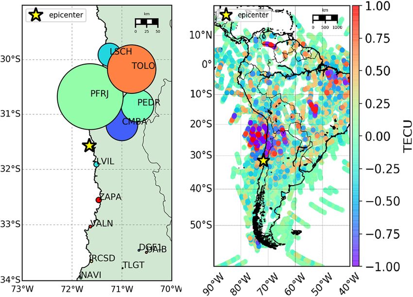
www.nature.com/scientificreports/
Figure 2. Upper panel—Real-time scenario estimated ground motion (Up component) through VADASE.
Bottom panels—sTEC variations for all the satellites in view for all the GPS stations computed through
VARION in range of 1500 km from the epicenter (left panel) and a zoom in the range of 150 km (right panel). In
both cases, positive and negative distances represent respectively the IPP position at 8 min after the earthquake
placed north and south the epicenter.
calculated by some a priori models (e.g. the International Reference Ionosphere—IRI—2016 model56,57 and
NeQuick model58,59—Fig. 6). We finally selected the NeQuick model because the computational time is faster
then IRI, giving a great advantage for the real-time aproach. Anyway, we highlight that the two models are fully
consistent. NeQuick model is based on a single input parameter—the Effective Ionisation Level (Az)—determined
using three coefficients broadcast in the Galileo navigation message60; this resulted, for the day of the Chile event,
in a maximum electron density height of 290 km.
The TEC time series were analysed with VARION during the time window from 21:45:00 to 23:59:59 GNSS
time. The longer period (> 35–40 min) component of the TEC variation was removed using an 8th order poly-
nomial fit in order to highlight the AGWepi29. We highlight that—in our knowledge—this is the first time that
the AGWepi is detected in a near real-time scenario.
Scientific Reports | (2021) 11:3114 | https://doi.org/10.1038/s41598-021-82532-6 4
Vol:.(1234567890)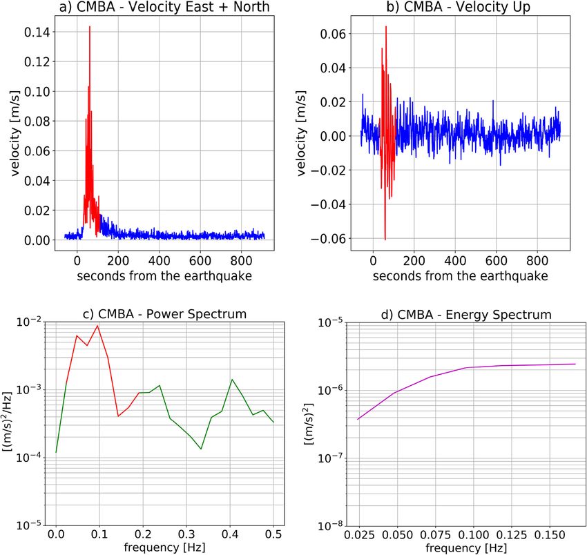
www.nature.com/scientificreports/
Figure 3. (a, b) Velocity time series for CMBA GPS station placed north of the epicenter. Specifically, (a)
and (b) show the horizontal component and the Up component of the velocity respectively. The duration
was computed on the horizontal component and then applied to the Up component of velocity. The red part
highlights the earthquake duration detected with the Levene test. (c) The PSD for CMBA station. In red the
chosen frequency range (3.3–200 mHz) for the integration. (d) The kinetic energy spectrum due to shaking in
vertical direction for CMBA station.
The elevation cut-off angle of 20◦ was used in order to remove the noisier observations as usually suggested
in the l iterature2. The bottom panels of Fig. 2 (the right panel is a zoom in of the green rectangle of the left one)
give a general vision of sTEC time series variations for all satellites and all stations, referred to the respective
IPP positions 8 min after the earthquake, and sorted by the IPP corresponding distances (positive and nega-
tive distances represent respectively the IPP placed north and south of the epicenter from the epicenter at this
epoch). It is important to highlight that overall 11 GPS satellites (G02, G05, G06, G12, G13, G14, G15, G20,
G24, G25, G29) observed from the 118 GPS permanent stations showing the much higher spatial coverage of
the ionospheric observations (bottom panels of Fig. 2) compared to the GNSS ground motion observation only
(upper panel of Fig. 2). The right panel of Fig. 4 shows the area analysed in which the coloured tracks represent
the sTEC variations at the SIPs (same positions of the corresponding IPPs projected on the Earth ellipsoid) from
the earthquake time (22:54:49 GPS time) to 23:59:59 GPS time. The TEC perturbation computed in real-time
by VARION and showed in the right panel of Fig. 4 is characterized by a favorable coverage and is consistent
with the source extent, proving the potential advantages to use real-time sTEC observations for tsunami genesis
estimation. Additionally, sTEC observations appear to correlate well with the vertical ground motion and the
related kinetic energy showing a strong perturbation mainly located at the North of the epicenter. Video S1 in
Supplementary Material shows the TEC perturbation appearing about 9.5 min after the earthquake and moving
northward.
The remarkable spatial density of ionospheric TEC observation by GNSS compared to ground motion (shown
in Figs. 2 and 4) is simply related to fact that ground information is calculated only at the GNSS station location,
instead the TEC measurements are located at the IPP between the GNSS station and the satellites. Consequently,
Scientific Reports | (2021) 11:3114 | https://doi.org/10.1038/s41598-021-82532-6 5
Vol.:(0123456789)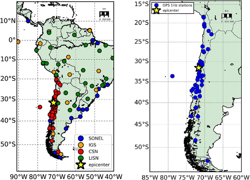
www.nature.com/scientificreports/
Figure 4. Left panel—Map of the earthquake ground shaking: the dimension of the station markers is
proportional to the energy associated to the Up component of the earthquake ground shaking for some stations
near the epicenter. It is evident that north placed stations are characterized by a higher energy than south placed
ones. Right panel—Space-time sTEC variations at the SIPs for less than two hours (22:54:49-23:59:59 GPS time)
on 16th September 2015 for all the satellites in view (cut-off angle set to 20◦ ) from all the 118 GPS stations.
East North Up
Stations Distance value σ value σ value σ Energy
– km cm cm cm cm cm cm J/kg
CMBA 76.91 − 76.76 0.13 0.28 0.62 − 13.56 1.88 2.45 e−6
PFRJ 99.33 − 137.98 0.12 − 19.77 0.57 − 10.36 1.72 5.09 e−6
North PEDR 124.01 − 49.50 0.13 − 6.38 0.58 − 1.81 1.75 2.52 e−6
TOLO 176.02 − 27.79 0.12 − 12.63 0.56 − 1.77 1.71 3.74 e−6
LSCH 188.73 − 18.56 0.14 − 10.23 0.64 4.81 1.94 1.80 e−6
LVIL 40.56 − 33.97 0.11 4.05 1.11 -9.01 1.79 4.02e−7
ZAPA 110.74 − 4.59 0.01 − 1.50 0.95 − 10.04 1.53 4.22 e−7
South VALN 161.71 − 1.98 0.15 − 5.14 1.41 2.69 2.28 2.21 e−7
DGF1 229.89 − 4.73 0.10 4.23 0.99 9.97 1.60 1.47 e−7
RCSD 231.23 − 2.16 0.09 − 0.16 0.87 2.41 1.40 1.98 e−7
Table 1. Overall coseismic displacements and their standard deviations for the GPS stations within 300 km
from the epicenter. The last column shows the value for the energy connected to the Up component of the
earthquake ground shaking.
at each epoch, every GNSS station has one single measurement of ground motion but several sTEC measure-
ments: nominally, one for each satellite in view. The actual multiplication of GNSS systems—i.e., GPS (US),
GLONASS (Russia), Galileo (EU), BeiDou (China)—is opening ambitious perspectives for really dense coverage
of ionospheric monitoring to support conventional ground motion observation by seismometers.
Figure 7 summarizes more than one hour (from 22:45:00 to 23:59:59 GPS time) of GNSS sTEC observa-
tions around the epicenter (hodochrones) and clearly shows the propagation of the AGWepi all around from
the epicenter at the speed of sound. The propagation speed of the AGWepi was estimated by linear least-squares
regression and the horizontal disturbance propagation velocities are estimated with their standard deviations
within the range of 620–640 m/s +/− 40 m/s (see Method for comparison with models). To better illustrate the
correspondence between vertical ground shaking and ionospheric sTEC disturbances, the area was divided into
six zones, four mainly on land and two mainly on the Pacific Ocean. The oblique straight lines, separating regions
3 and 4, and regions 5 and 6, have azimuths respectively equal to 45 and 135 degrees. We selected the satellites
with the best observation geometry well highlighting the sTEC perturbation (other satellites are showed in the
Fig. SM5). As expected, and coherently with the ground motion observations, the TEC perturbations are more
evident in the north of the epicenter (region 1, 3 and 4). This effect is also partially induced by the magnetic
field lines18,61.
Scientific Reports | (2021) 11:3114 | https://doi.org/10.1038/s41598-021-82532-6 6
Vol:.(1234567890)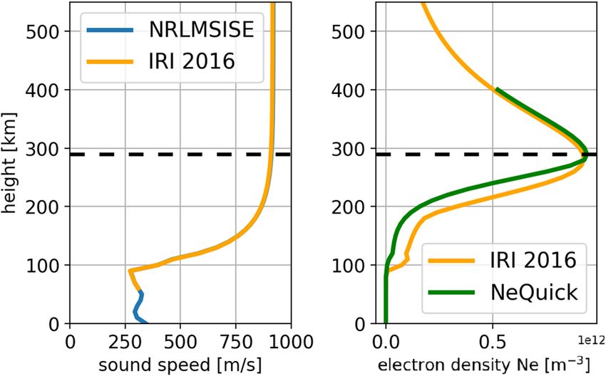
www.nature.com/scientificreports/

                                  Figure 5.  VADASE detrended coseismic displacements for the East (a), North (b) and Up (c) component. The
                                  stations are ordered according to their distance from the epicenter (positive distances for north placed stations
                                  and negative distances for south placed stations). The spatial median computed for the north and south stations
                                  is depicted in black; the red part highlights the interval over which the robust linear fit was estimated, whereas
                                  the dashed line represents the extrapolated trend.

Scientific Reports |   (2021) 11:3114 |                https://doi.org/10.1038/s41598-021-82532-6                                                  7

                                                                                                                                              Vol.:(0123456789)
www.nature.com/scientificreports/
Figure 6. Sound velocity (right) and electron density profile (left) with altitude on September 16th 2015
according to IRI 2016 and Nequick model.
Conclusions
VADASE and VARION variometric algorithms were defined and implemented in the past years to estimate
ground shaking, co-seismic displacements and ionosphere disturbances from GNSS data in real time. In this
paper we combined the two algorithms in a single one so-called Total Variometric Approach (TVA); only GNSS
data that are really available in real time were analized in a real-time scenario with TVA to retrieve the ground
shaking, the energy associated to its Up component and the ionospheric signature due to the September 16,
2015 Mw 8.3 Illapel earthquake in Chile. We highlight that both ground-motion and TEC measurements reveal
the north-south asymmetry related to the geometry of the rupture, and coherently with the plate tectonic local
characteristic.
The proposed real-time Total Variometric Approach (TVA) provides us with both ground shaking and TEC
perturbation in real time, on the basis of the same GNSS data stream. The TVA applied to the case of study
of the Illapel earthquake (Mw 8.3, Chile) in 2015 using the data stream of 118 GNSS stations all around the
epicenter allows to estimate significant ground shaking at only 30 s after the rupture as well as the consequent
energy related to the shaking. Additionally, the anomalous TEC perturbation, estimated with the same GNSS
data-stream, and related to the propagation of the AGWepi , is detected at 9.5 min after the rupture and it also
displays the north-south asymmetry previously shown by the GNSS ground-motion measurements. The high
spatial resolution of the GNSS-TEC observations reveal the source extent, the potential advantages introduced
by the ionospheric observations. We highlight that no classic techniques are today able to directly measure the
source extent of the rupture during an earthquake.
Therefore, for the very first time, we have demonstrated to simultaneously monitor—using the Total Vari-
ometric Aproach (TVA) on the same real-time GNSS data-stream—the ground-motion and the ionospheric
TEC perturbation to support traditional instrument (e.g., seismometers, accelerometers, buoys and tide gages)
to improve the quick estimation of the source parameters and to estimate the tsunami genesis.
Considering the richness of the information coming from ionospheric sounding and the demonstrated pos-
sibility to detect the ionospheric perturbation related to the AGWepi in about 9.5 min, TVA can be already used
for to support classic tsunami warning system. Indeed, following Manta et al.16 the ionospheric tsunami power
index (ITPI) of the Illapel event in 2015 is 14.51, corresponding to the estimated water-volume in the order of
104 km3 displaced during the tsunami genesis.
Consequently, the final goal of the paper is to underline the feasibility and reliability of TVA approach for
tsunami detection. Indeed, the TVA main advantages is to leverage the information coming from the ionosphere
to densify the GNSS observations and to make up for the lack of any other data. This makes TVA suitable for
regions without high GNSS coverage (e.g., Sumatra and Pacific region) or a massive scientific infrastructure (e.g.,
supercomputers). Furthermore, TVA represents a low-cost tool, ready to be implemented on existing high-rate
GNSS real-time networks and to push forward the installation of new dense GNSS real-time networks. Finally,
TVA main goal is to represent an additional resource to classic methods, such as tsunami forecast62, earthquake
early warning for tsunami a lert63, tsunami inundation simulation and damage e stimation64,65; in this context,
the synergic use of all the available tools could really enhance the already existing tsunami warning systems.
Methods
Total Variometric Approach The proposed real-time method is called Total Variometric Approach (TVA) and it
is based on the joint use of VARION and VADASE algorithms. Both algorithms share the same variometric prin-
ciple (time single-difference of proper combinations of phase observations) using a standalone GPS receiver and
standard GNSS broadcast products (orbits and clock corrections) that are available in real-time; VADASE uses
ionosphere-free combination and it estimates GNSS station velocities and displacements (thus earthquake ground
shaking)41,42, while VARION uses geometry-free combination and it estimates sTEC variations29. VADASE and
VARION can run in parallel but independently using the same GNSS data stream, so that TVA represents a com-
prehensive way to GNSS ground and ionosphere seismology, ready to be implemented on still existing high-rate
Scientific Reports | (2021) 11:3114 | https://doi.org/10.1038/s41598-021-82532-6 8
Vol:.(1234567890)www.nature.com/scientificreports/
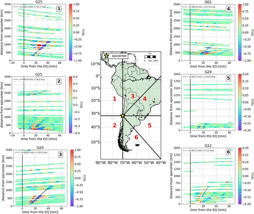
Figure 7. Map indicating the division in six regions of the studied area making the epicenter the area center.
The two western sectors (1 and 2) are mainly placed over the Pacific Ocean, while the four eastern sectors (3, 4, 5
and 6) are mainly placed over land. Hodochron plots for the 6 regions identified computed for a time interval of
one hour and 15 min (from 22:45:00 to 23:59:59 GPS time) and for some satellites in view (cut-off angle of 20◦ )
from all the 118 GPS stations. The number in the upper right box denotes the region to which the hodochrones
belong. The slope of the straight line fitted, considering a linear least-squares regression for corresponding sTEC
minima for different satellites, represent the AGWepi horizontal propagation velocity.
GNSS permanent networks able to supply real-time data. Here data processing with both VADASE and VARION
was performed off-line, even if in a real-time scenario: exclusively the information available in real time was used.
VADASE starting from the previous developed and published m ethodology41,42, the algorithm was improved
with statistical test to define the significant shaking duration on the basis of the mean noise level of the velocity
components, which have been recognized to be constant before and after the earthquake shaking generally with
Gaussian distribution. East, North and Up velocities before and after the earthquake were evaluated to determine
whether data are normally distributed. The result from D’Agostino–Pearson66 test shows that the data follows a
Gaussian distribution as shown in Fig. SM6 of the Supplementary material. The incidence of non-normality is
equal at most to 12.5%. For this reason, Levene test for equality of variances67 was chosen instead of the F-test
applied in Fratarcangeli et al.42: Levene test is, indeed, less powerful, but, at the same time, less sensitive to
departure from normality than F-test. The Levene test was performed on the horizontal velocity component
(sum of East and North components).
Starting from the duration of significant shaking, we defined the overall coseismic displacements and the
energy released by the earthquake. The series of the coseismic displacements, computed from the integration
of VADASE velocity solutions, for the East, North and Up component, were de-trended as follows. First, we
computed the spatial median of the displacements for the stations within 300 km of the epicenter as reported in
Fratarcangeli et al.42. In our case, we computed two different medians—respectively for the northward and the
Scientific Reports | (2021) 11:3114 | https://doi.org/10.1038/s41598-021-82532-6 9
Vol.:(0123456789)www.nature.com/scientificreports/
southward stations—since they are impacted differently by the rupture. The spatial median was fitted robustly
with a linear model (Huber regression m odel68) considering the interval of 60 s before the earthquake for the
nearest stations (CMBA in the north and LVIL in the south). This straight line was extrapolated on all the
interval of the coseismic displacements and then removed. Once completed the de-trending procedure, the
overall coseismic displacements were computed using the strategy reported in Fratarcangeli et al.42. Based on
the de-trending estimation, we also determined the uncertainty (sigmas) on the coseismic displacements using
the model reported in Equation 1. More in detail, Cr represents the overall coseismic displacements estima-
tion; a and b are respectively the slope and y-intercept of the robusted estimated linear model; σa2, σb2 and σab are
the variances of the slope and y-intercept and the covariance between a and b respectively; t is the significant
shaking duration.
Regarding the energy produced by the Up component of ground shaking released by the earthquake, we
computed the Power Spectral Density (PSD) to the ground shaking duration for the up component of the velocity
at each site. The PSD was estimated using Welch method: an improvement of the standard periodogram spec-
trum estimation method, able to reduce the noise in the estimated power spectra in exchange for reducing the
frequency resolution69,70. By integrating the PSD within a specific frequency range, the energy (in that frequency
range) was calculated. This range is limited below by the specific cut-off frequency for the AGWepi , as reported
in the Introduction section. In this way, the normalized (for unit mass) kinetic energy for the Up component,
related to the earthquake shaking, was computed for each site.
σ 2 σ �t
σ�2 Cr = �t 1 a ab2
σab σ 1 (1)
b
Atmospheric velocity of AGWepi The estimated velocity of the AGWepi by the analysis of Fig. 7 were also vali-
dated with the US Naval Research Laboratory Mass-Spectrometer Incoherent-Scatter (NRL MSISE-00) and
IRI-2016 models. The NRL MSISE-00 is an empirical, global model of the Earth’s atmosphere from ground to
thermospheric heights whose outputs are temperatures and densities of the atmosphere c omponents71. Hence,
the temperature
T profile as a function of the height in the earthquake day was computed. Then the sound veloc-
ity, cs = γmTR 1
, where R (approximately 8.3145 J mol−1 K−1), is the molar gas constant, γ is the adiabatic index
(1.6667 for monatomic gases and 1.4 for diatomic gases), and m1 is the molar mass of the gases, was evaluated.
The left panel of Fig. 6 shows the sound velocity profile for the earthquake day: a velocity of about 910 m/s is
estimated at an height of 290 km (F2 layer height, where the electron density is maximum). This sound velocity
derived from model is coherent with the estimated sTEC perturbations velocity range, since hodochrones rep-
resent only the horizontal propagation velocity component of the AGWepi at the level of the F2 maximum, not
the full velocity along the propagating k-vector.
Received: 3 September 2020; Accepted: 20 January 2021
References
1. Occhipinti, G. The seismology of the planet mongo: the 2015 ionospheric seismology review. In Subduction Dynamics: From Mantle
Flow to Mega Disasters (eds Morra, G. et al.) 169–182 (Wiley, Hoboken, 2015).
2. Occhipinti, G., Rolland, L., Lognonné, P. & Watada, S. From Sumatra 2004 to Tohoku-Oki 2011: the systematic GPS detection of the
ionospheric signature induced by tsunamigenic earthquakes. J. Geophys. Res. Space Phys. 118, 3626–3636. https://doi.org/10.1002/
jgra.50322(2013).
3. Tanimoto, T. Interaction of solid earth, atmosphere, and ionosphere. Treatise Geophys. 4, 421–444 (2007).
4. Artru, J., Farges, T. & Lognonné, P. Acoustic waves generated from seismic surface waves: propagation properties determined from
Doppler sounding observations and normal-mode modelling. Geophys. J. Int. 158, 1067–1077. https://doi.org/10.1111/j.1365-
246X.2004.02377.x (2004).
5. Chum, J. et al. Ionospheric signatures of the April 25, 2015 Nepal earthquake and the relative role of compression and advection
for Doppler sounding of infrasound in the ionosphere. Earth Planets Space 68, 24. https://doi.org/10.1186/s40623-016-0401-9
(2016).
6. Hickey, M., Schubert, G. & Walterscheid, R. Atmospheric airglow fluctuations due to a tsunami-driven gravity wave disturbance.
J. Geophys. Res. Space Phys. 115, A06308 (2010).
7. Makela, J. et al. Imaging and modeling the ionospheric airglow response over Hawaii to the tsunami generated by the Tohoku
earthquake of 11 March 2011. Geophys. Res. Lett. 38, L00G02 (2011).
8. Occhipinti, G., Dorey, P., Farges, T. & Lognonné, P. Nostradamus: the radar that wanted to be a seismometer. Geophys. Res. Lett.
37, L18104 (2010).
9. Occhipinti, G., Aden-Antoniow, F., Bablet, A., Molinie, J.-P. & Farges, T. Surface waves magnitude estimation from ionospheric
signature of Rayleigh waves measured by Doppler sounder and OTH radar. Sci. Rep. 8, 1555. https://doi.org/10.1038/s41598-018-
19305-1 (2018).
10. Calais, E., Bernard Minster, J., Hofton, M. & Hedlin, M. Ionospheric signature of surface mine blasts from global positioning
system measurements. Geophys. J. Int. 132, 191–202. https://doi.org/10.1046/j.1365-246x.1998.00438.x (1998).
11. Astafyeva, E., Heki, K., Kiryushkin, V., Afraimovich, E. & Shalimov, S. Two-mode long-distance propagation of coseismic iono-
sphere disturbances. J. Geophys. Res. Space Phys. https://doi.org/10.1029/2008JA013853 (2009).
12. Astafyeva, E. & Heki, K. Dependence of waveform of near-field coseismic ionospheric disturbances on focal mechanisms. Earth
Planets Space 61, 939–943. https://doi.org/10.1186/BF03353206 (2009).
13. Ducic, V., Artru, J. & Lognonné, P. Ionospheric remote sensing of the Denali earthquake Rayleigh surface waves. Geophys. Res.
Lett. https://doi.org/10.1029/2003GL017812 (2003).
14. Mannucci, A. J., Wilson, B. D. & Edwards, C. D. A new method for monitoring the Earth’s ionospheric total electron content
using the GPS global network. In Proceedings of the 6th International Technical Meeting of the Satellite Division of the Institute of
Navigation (ION GPS 1993), 1323–1332 (September, 1993).
Scientific Reports | (2021) 11:3114 | https://doi.org/10.1038/s41598-021-82532-6 10
Vol:.(1234567890)www.nature.com/scientificreports/
15. Mannucci, A. et al. A global mapping technique for GPS-derived ionospheric total electron content measurements. Radio Sci. 33,
565–582 (1998).
16. Manta, F., Occhipinti, G., Feng, L. & Hill, E. Rapid identification of tsunamigenic earthquakes using GNSS ionospheric sounding.
Sci. Rep. 10, 11054. https://doi.org/10.1038/s41598-020-68097-w (2020).
17. Occhipinti, G., Lognonné, P., Kherani, E. A. & Hébert, H. Three-dimensional waveform modeling of ionospheric signature induced
by the 2004 Sumatra tsunami. Geophys. Res. Lett. https://doi.org/10.1029/2006GL026865 (2006).
18. Occhipinti, G., Komjathy, A. & Lognonné, P. Tsunami detection by GPS. GPS World 19, 51–57 (2008).
19. Occhipinti, G. et al. Three-dimensional numerical modeling of tsunami-related internal gravity waves in the Hawaiian atmosphere.
Earth Planets Space 63, 847–851 (2011).
20. Rolland, L. M., Occhipinti, G., Lognonné, P. & Loevenbruck, A. Ionospheric gravity waves detected offshore Hawaii after tsunamis.
Geophys. Res. Lett. https://doi.org/10.1029/2010GL044479 (2010).
21. Heki, K. Explosion energy of the 2004 eruption of the Asama volcano, central Japan, inferred from ionospheric disturbances.
Geophys. Res. Lett. 33, L14303 (2006).
22. Dautermann, T., Calais, E. & Mattioli, G. S. Global positioning system detection and energy estimation of the ionospheric wave
caused by the 13 July 2003 explosion of the Soufrière Hills Volcano. Montserrat. J. Geophys. Res. Solid Earth 114, B02202 (2009).
23. Nakashima, Y. et al. Atmospheric resonant oscillations by the 2014 eruption of the Kelud volcano, Indonesia, observed with the
ionospheric total electron contents and seismic signals. Earth Planet. Sci. Lett. 434, 112–116 (2016).
24. Jacobson, A. R., Carlos, R. C. & Blanc, E. Observations of ionospheric disturbances following a 5-kt chemical explosion 1. Persistent
oscillation in the lower thermosphere after shock passage. Radio Sci. 23, 820–830 (1988).
25. Huang, C. Y., Helmboldt, J., Park, J., Pedersen, T. & Willemann, R. Ionospheric detection of explosive events. Rev. Geophys. 57,
78–105 (2019).
26. Booker, H. G. A local reduction of f-region ionization due to missile transit. J. Geophys. Res. 66, 1073–1079 (1961).
27. Mendillo, M., Hawkins, G. S. & Klobuchar, J. A. A sudden vanishing of the ionospheric F region due to the launch of skylab. J.
Geophys. Res. 80, 2217–2228 (1975).
28. Savastano, G. et al. Advantages of geostationary satellites for ionospheric anomaly studies: ionospheric plasma depletion following
a rocket launch. Remote Sens. 11, 1734 (2019).
29. Savastano, G. et al. Real-time detection of tsunami ionospheric disturbances with a stand-alone GNSS receiver: a preliminary
feasibility demonstration. Sci. Rep. 7, 46607. https://doi.org/10.1038/srep46607 (2017).
30. Savastano, G. & Ravanelli, M. Real-time monitoring of ionospheric irregularities and tec perturbations. In Satellites Missions and
Technologies for Geosciences (eds Demyanov, V. & Becedas, J.) (IntechOpen, Rijeka, 2019). https://doi.org/10.5772/intechopen
.90036.
31. Blewitt, G. et al. Rapid determination of earthquake magnitude using GPS for tsunami warning systems. Geophys. Res. Lett. 33,
L11309 (2006).
32. Kouba, J. Measuring seismic waves induced by large earthquakes with gps. Studia Geophys. et Geod. 47, 741–755 (2003).
33. Langbein, J. & Bock, Y. High-rate real-time GPS network at Parkfield: utility for detecting fault slip and seismic displacements.
Geophys. Res. Lett. 31, L15S20 (2004).
34. Larson, K. M., Bilich, A. & Axelrad, P. Improving the precision of high-rate GPS. J. Geophys. Res. Solid Earth 112, B05422 (2007).
35. Larson, K. M. Gps seismology. J. Geod. 83, 227–233 (2009).
36. Ohta, Y. et al. Quasi real-time fault model estimation for near-field tsunami forecasting based on RTK-GPS analysis: application
to the 2011 Tohoku-Oki earthquake (Mw 90). J. Geophys. Res. Solid Earth 117, B02311 (2012).
37. Melgar, D. et al. Earthquake magnitude calculation without saturation from the scaling of peak ground displacement. Geophys.
Res. Lett. 42, 5197–5205 (2015).
38. Melgar, D., Bock, Y. & Crowell, B. W. Real-time centroid moment tensor determination for large earthquakes from local and
regional displacement records. Geophys. J. Int. 188, 703–718 (2012).
39. Crowell, B. W., Bock, Y. & Melgar, D. Real-time inversion of GPS data for finite fault modeling and rapid hazard assessment.
Geophys. Res. Lett. 39, L09305 (2012).
40. Allen, R. M. & Melgar, D. Earthquake early warning: advances, scientific challenges, and societal needs. Annu. Rev. Earth Planet.
Sci. 47, 361–388 (2019).
41. Colosimo, G., Crespi, M. & Mazzoni, A. Real-time GPS seismology with a stand-alone receiver: a preliminary feasibility demon-
stration. J. Geophys. Res. Solid Earth https://doi.org/10.1029/2010JB007941 (2011).
42. Fratarcangeli, F. et al. Vadase reliability and accuracy of real-time displacement estimation: Application to the central Italy 2016
earthquakes. Remote Sens. https://doi.org/10.3390/rs10081201 (2018).
43. USGS. Earthquake Hazard Program. https://earthquake.usgs.gov/earthquakes/eventpage/us20003k7a/executive (2019).
44. NOAA/National Weather Service. Event Messages. https://www.tsunami.gov/php/prevEventresults.php?start_date=2015-09-
16&end_date=2015-09-16&bulletin_count=&Submit=Invia (2020).
45. UNESCO. International Tsunami Information Center. http://itic.ioc-unesco.org/index.php?option=com_content&view=artic
le&id=1946:16-september-2015-utc-mw-8-3-northern-chile-tsunami&catid=2164&Itemid=2616 (2020).
46. ARMADA DE CHILE. SHOA difunde oportuna Alerta de Tsunami. https://www.armada.cl/armada/noticias-navales/shoa-difun
de-oportuna-alerta-de-tsunami/2015-09-17/103011.html, https://www.armada.cl/armada/comunicados/en-solo-8-minutos-el-
shoa-entrego-alerta-de-tsunami-tras-terremoto/2015-09-17/111514.html (2020).
47. NOAA. NATIONAL CENTER FOR ENVIRONMENTAL INFORMATION. https://www.ngdc.noaa.gov/nndc/struts/resul
ts?EQ_0=5590&t=101650&s=9&d=100,91,95,93&nd=display (2015).
48. NOAA. NATIONAL CENTER FOR ENVIRONMENTAL INFORMATION. https://www.ngdc.noaa.gov/nndc/struts/resul
ts?EQ_0=5590&t=101650&s=9&d=92,183&nd=display (2015).
49. NOAA, NWS NATIONAL TSUNAMI WARNING CENTER PALMER AK. PUBLIC TSUNAMI MESSAGE NUMBER 22. https
://www.tsunami.gov/events/PAAQ/2015/09/16/nuskyv/22/WEAK51/WEAK51.txt (2015).
50. RTCM. Radio Technical Commission for Maritime Services. https://www.rtcm.org/ (2020).
51. GNSS Science Support Centre, ESA. Networked Transport of RTCM via Internet Protocol. https://gssc.esa.int/wp-content/uploa
ds/2018/07/NtripDocumentation.pdf (2020).
52. Vincenty, T. Direct and inverse solutions of geodesics on the ellipsoid with application of nested equations. Surv. Rev. 23, 88–93.
https://doi.org/10.1179/sre.1975.23.176.88 (1975).
53. World Data Center for Geomagnetism. Kyoto. http://wdc.kugi.kyoto-u.ac.jp/index.html (2018).
54. NOAA. Space Weather Prediction Center. http://www.swpc.noaa.gov/products/planetary-k-index (2018).
55. Loewe, C. & Prölss, G. Classification and mean behavior of magnetic storms. J. Geophys. Res. Space Phys. 102, 14209–14213. https
://doi.org/10.1029/96JA04020 (1997).
56. Committee on Space Research and the International Union of Radio Science. International Reference Ionosphere. http://irimodel.
org/ (2020).
57. Haystack Observatory, MIT. Realtime IRI. http://madrigal.haystack.mit.edu/models/IRI/index.html (2018).
58. International Centre for Theoretical Physics. NeQuick Model. https://t-ict4d.ictp.it/nequick2 (2020).
59. Nava, B., Radicella, S., Leitinger, R. & Coïsson, P. A near-real-time model-assisted ionosphere electron density retrieval method.
Radio Sci. 41, RS6S16 (2006).
Scientific Reports | (2021) 11:3114 | https://doi.org/10.1038/s41598-021-82532-6 11
Vol.:(0123456789)www.nature.com/scientificreports/
60. European GNSS (Galileo) Open Service. Ionospheric Correction Algorithm for Galileo Single Frequency Users. www.gsc-europa.eu/
sites/default/files/sites/all/files/Galileo_Ionospheric_Model.pdf (2016).
61. Rolland, L. M., Lognonné, P. & Munekane, H. Detection and modeling of rayleigh wave induced patterns in the ionosphere. J.
Geophys. Res. Space Phys. https://doi.org/10.1029/2010JA016060 (2011).
62. Ohta, Y., Inoue, T., Koshimura, S., Kawamoto, S. & Hino, R. Role of real-time GNSS in near-field tsunami forecasting. J. Disaster
Res. 13, 453–459 (2018).
63. Crowell, B. W. et al. G-fast earthquake early warning potential for great earthquakes in Chile. Seismol. Res. Lett. 89, 542–556 (2018).
64. Kawamoto, S. et al. Regard: a new GNSS-based real-time finite fault modeling system for GEONET. J. Geophys. Res. Solid Earth
122, 1324–1349 (2017).
65. Musa, A. et al. Real-time tsunami inundation forecast system for tsunami disaster prevention and mitigation. J. Supercomput. 74,
3093–3113 (2018). √
66. D’Agostino, R. & Pearson, E. S. Tests for departure from normality. Empirical results for the distributions of b 2 and b . Biometrika
60, 613–622. https://doi.org/10.1093/biomet/60.3.613 (1973).
67. Levene, H. Robust Tests for Equality of Variances. Contributions to probability statistics. In: Essays honor Harold Hotelling, 279–292
(1961).
68. Huber, P. J. & Ronchetti, E. M. Robust statistics Vol. 1 (Wiley, New York, 1981).
69. Buttkus, B. Spectral Analysis and Filter Theory in Applied Geophysics (Springer, Berlin, 2012).
70. Welch, P. The use of fast Fourier transform for the estimation of power spectra: a method based on time averaging over short,
modified periodograms. IEEE Trans. Audio Electroacoust. 15, 70–73. https://doi.org/10.1109/TAU.1967.1161901 (1967).
71. Picone, J., Hedin, A., Drob, D. P. & Aikin, A. Nrlmsise-00 empirical model of the atmosphere: statistical comparisons and scientific
issues. J. Geophys. Res. Space Phys. 107, SIA-5. https://doi.org/10.1029/2002JA009430 (2002).
Acknowledgements
The authors are grateful to Juan Carlos Baez and Felipe Leyton from Centro Sismológico Nacional, Universidad de
Chile for providing valuable GPS and accelerometer data and precious information. This research was partially
supported by Sapienza University of Rome, through PhD fellowships granted to Michela Ravanelli. A portion
of this research was carried out at the Jet Propulsion Laboratory, California Institute of Technology, under a
contract with the National Aeronautics and Space Administration. G.O. is supported by Programme National
de Télédétection Spatiale (PNTS), grant n PNTS-2014-07; by the CNES, grant GISnet&Back; and by the Institut
Universitaire de France (IUF). M.C. was partially supported by a grant from IPGP.
Author contributions
M.C., M.R. and G.S. conceived the work; M.R conducted all the analysis and produced the Figures; M.R., G.O.
and M.C. wrote the draft; M.R., G. O., A.K., E.S. G.S., M.C., discussed the results. All authors reviewed the
manuscript.
Competing interests
The authors declare no competing interests.
Additional information
Supplementary Information The online version contains supplementary material available at https://doi.
org/10.1038/s41598-021-82532-6.
Correspondence and requests for materials should be addressed to M.R.
Reprints and permissions information is available at www.nature.com/reprints.
Publisher’s note Springer Nature remains neutral with regard to jurisdictional claims in published maps and
institutional affiliations.
Open Access This article is licensed under a Creative Commons Attribution 4.0 International
License, which permits use, sharing, adaptation, distribution and reproduction in any medium or
format, as long as you give appropriate credit to the original author(s) and the source, provide a link to the
Creative Commons licence, and indicate if changes were made. The images or other third party material in this
article are included in the article’s Creative Commons licence, unless indicated otherwise in a credit line to the
material. If material is not included in the article’s Creative Commons licence and your intended use is not
permitted by statutory regulation or exceeds the permitted use, you will need to obtain permission directly from
the copyright holder. To view a copy of this licence, visit http://creativecommons.org/licenses/by/4.0/.
© The Author(s) 2021
Scientific Reports | (2021) 11:3114 | https://doi.org/10.1038/s41598-021-82532-6 12
Vol:.(1234567890)You can also read