IAB-DISCUSSION PAPER 10|2021 Lockdown length and strength: labour-market effects in Germany during the COVID-19 pandemic

IAB-DISCUSSION PAPER
Articles on labour market issues

10|2021Lockdown length and strength:
labour-market effects in Germany during the
COVID-19 pandemic

Anja Bauer, Enzo Weber

 ISSN 2195-2663

Lockdown length and strength:
labour-market effects in Germany during the
COVID-19 pandemic

Anja Bauer (IAB),
Enzo Weber (IAB, University of Regensburg)

Mit der Reihe „IAB-Discussion Paper“ will das Forschungsinstitut der Bundesagentur für Ar-
beit den Dialog mit der externen Wissenschaft intensivieren. Durch die rasche Verbreitung
von Forschungsergebnissen über das Internet soll noch vor Drucklegung Kritik angeregt und
Qualität gesichert werden.

The “IAB-Discussion Paper” is published by the research institute of the German Federal Em-
ployment Agency in order to intensify the dialogue with the scientific community. The prompt
publication of the latest research results via the internet intends to stimulate criticism and to
ensure research quality at an early stage before printing.

Contents

1 Introduction . . . . . . . . . . . . . . . . . . . . . . . . . . . . . . . . . . . . . . . . . . . . . . . . . . . . . . . . . . . . . . . . . . . . . . . . . . . . . . . . . . . . 7

2 Germany in the first wave of the pandemic . . . . . . . . . . . . . . . . . . . . . . . . . . . . . . . . . . . . . . . . . . . . . . . . . 8

3 Impact Channel: Lockdown length. . . . . . . . . . . . . . . . . . . . . . . . . . . . . . . . . . . . . . . . . . . . . . . . . . . . . . . . . 10

4 Impact Channel: Lockdown strength . . . . . . . . . . . . . . . . . . . . . . . . . . . . . . . . . . . . . . . . . . . . . . . . . . . . . . 16

5 Short-time work . . . . . . . . . . . . . . . . . . . . . . . . . . . . . . . . . . . . . . . . . . . . . . . . . . . . . . . . . . . . . . . . . . . . . . . . . . . . . . 19

6 Robustness. . . . . . . . . . . . . . . . . . . . . . . . . . . . . . . . . . . . . . . . . . . . . . . . . . . . . . . . . . . . . . . . . . . . . . . . . . . . . . . . . . . . 21
 6.1 Robustness on length . . . . . . . . . . . . . . . . . . . . . . . . . . . . . . . . . . . . . . . . . . . . . . . . . . . . . . . . . . . . . . . . . . .21
 6.2 Robustness on strength . . . . . . . . . . . . . . . . . . . . . . . . . . . . . . . . . . . . . . . . . . . . . . . . . . . . . . . . . . . . . . . . .22
 6.2.1 Timing of events . . . . . . . . . . . . . . . . . . . . . . . . . . . . . . . . . . . . . . . . . . . . . . . . . . . . . . . . . . . . . . . .23
 6.2.2 Back-of-the-envelope calculations. . . . . . . . . . . . . . . . . . . . . . . . . . . . . . . . . . . . . . . . . . . .23

7 Conclusion . . . . . . . . . . . . . . . . . . . . . . . . . . . . . . . . . . . . . . . . . . . . . . . . . . . . . . . . . . . . . . . . . . . . . . . . . . . . . . . . . . . . 24
 References . . . . . . . . . . . . . . . . . . . . . . . . . . . . . . . . . . . . . . . . . . . . . . . . . . . . . . . . . . . . . . . . . . . . . . . . . . . . . . . . . . . . . .26

Appendix . . . . . . . . . . . . . . . . . . . . . . . . . . . . . . . . . . . . . . . . . . . . . . . . . . . . . . . . . . . . . . . . . . . . . . . . . . . . . . . . . . . . . . . . . . 27

8 Input-Output Linkage . . . . . . . . . . . . . . . . . . . . . . . . . . . . . . . . . . . . . . . . . . . . . . . . . . . . . . . . . . . . . . . . . . . . . . . . 27

9 Timing of events. . . . . . . . . . . . . . . . . . . . . . . . . . . . . . . . . . . . . . . . . . . . . . . . . . . . . . . . . . . . . . . . . . . . . . . . . . . . . . 29

List of Figures

Figure 1: Daily number of confirmed cases over time . . . . . . . . . . . . . . . . . . . . . . . . . . . . . . . . . . . . . . . . . . . 9
Figure 2: Persons in notifications of short-time work and unemployment over time.. . . . . . .10
Figure 3: Separation rate (left axis) and job-finding rate (right axis) across time. . . . . . . . . . . . .11
Figure 4: Average number of days of economic closures and curfews over time . . . . . . . . . . . .12
Figure 5: Average number of days of economic closures and curfews across federal states 13
Figure 6: Total and marginal effects of economic closures (solid lines) and curfews (dot-
 ted line) on separation rate (upper panel) and job-finding rate (lower panel) . . . . .15

IAB-Discussion Paper 10|2021 3

List of Tables

Table 1: Regression of labour market flows on closing days - Robustness Check. . . . . . . . . . . .14
Table 2: Regression of separations and hirings on degree of closure . . . . . . . . . . . . . . . . . . . . . . . . .18
Table 3: Regression of persons in short-time work on closing days and curfews . . . . . . . . . . . .19
Table 4: Regression of persons in short-time work on degree of closure . . . . . . . . . . . . . . . . . . . . .20
Table 5: Regression of labour market flows on closing days - Robustness Check. . . . . . . . . . . .21
Table 6: Regression of separations and hirings on degree of closure using input-output
 linkage . . . . . . . . . . . . . . . . . . . . . . . . . . . . . . . . . . . . . . . . . . . . . . . . . . . . . . . . . . . . . . . . . . . . . . . . . . . . . . . . . . . .22
Table 7: Inflows to unemployment from employment subject to social security contri-
 butions . . . . . . . . . . . . . . . . . . . . . . . . . . . . . . . . . . . . . . . . . . . . . . . . . . . . . . . . . . . . . . . . . . . . . . . . . . . . . . . . . . .27
Table 8: Regression of separations and hirings on degree of closure - reference month
 January . . . . . . . . . . . . . . . . . . . . . . . . . . . . . . . . . . . . . . . . . . . . . . . . . . . . . . . . . . . . . . . . . . . . . . . . . . . . . . . . . . .29

IAB-Discussion Paper 10|2021 4

Abstract

This paper evaluates the short-term labour market impact of the COVID-19 containment mea-
sures in Germany. It examines two dimensions of the first lockdown in Germany, namely the
length and the strength of the lockdown. While the assessment of the length is conducted
via variation across regions and time in closing days and curfews, the latter uses the degree
of closure in different sectors. For the length of the lockdown we find that an additional day
of closure lead to an increase in the separation rate of 2.7 percent and a decrease in the job-
finding rate of 1.8 percent. For the strength of the lockdown the results show that a higher
degree of closure increases separations and lower job findings to a similar extent. In both
dimensions, we find that the effects are non-linear over time. Given this approach, we find
that 31 percent of the considerably increased inflows from employment into unemployment,
and 33 percent of the reduced outflows from unemployment to employment in the first wave
were due to the treatment effect of the lockdown measures. In sum, the lockdown measures
increased unemployment in the short run by 80,000 persons.

Zusammenfassung

Dieses Papier evaluiert die kurzfristigen Arbeitsmarkteffekte der COVID-19-Eindämmungs-
maßnahmen in Deutschland. Wir untersuchen zwei verschiedene Dimensionen des ersten
Lockdowns in Deutschland, nämlich die Länge und die Stärke des Lockdowns. Während die
Länge über die regionale und zeitliche Variation der Schließungstage und Ausgangssperren
erfolgt, wird für die Stärke der Grad der Schließung in verschiedenen Branchen herangezo-
gen. Für die Länge des Lockdowns finden wir, dass ein zusätzlicher Tag zu einem Anstieg der
Entlassungsrate um 2,7 Prozent und einem Rückgang der Einstellungsrate um 1,8 Prozent
führt. Für die Stärke der Schließung zeigen die Ergebnisse, dass ein höherer Grad der Schlie-
ßung die Entlassungen erhöht und die Einstellungen in ähnlichem Ausmaß senkt. In beiden
Dimensionen stellen wir fest, dass die Effekte im Zeitverlauf nicht linear sind. Mit diesem An-
satz finden wir, dass 31 Prozent der deutlich erhöhten Zuflüsse aus Beschäftigung in Arbeits-
losigkeit und 33 Prozent der verringerten Abflüsse aus Arbeitslosigkeit in Beschäftigung in der
ersten Welle auf die Schließungsmaßnahmen zurückzuführen sind. In Summe erhöhten
die Eindämmungsmaßnahmen die Arbeitslosigkeit in der kurzen Frist um 80.000
Personen.

JEL

J6, E24

IAB-Discussion Paper 10|2021 5

Keywords

Keywords: containment measures, COVID-19, job finding rate, separation rate

Acknowledgements

We thank Maximilian Studtrucker and Katharina Vogel for excellent research assistance. Fur-
thermore we thank participants of the 17. IWH/IAB-Workshop, the DTMC COVID-19 Workshop
2020 and the RWI research seminar for valuable comments and suggestions.

IAB-Discussion Paper 10|2021 6

1 Introduction

In 2020, the Corona virus started to spread across the globe. All over the world governments
reacted by shutting down the economies. Now, in the beginning of 2021, the pandemic is
still ubiquitous,and though vaccines exist, a lot of countries faced a second or even third
shutdown over the course of the fall and winter. Meanwhile a lot is known so far about the
reactions of the economies on the containment measures. The literature, that emerged so
far, combines the epidemiologic workhorse model, the so-called SIR-model with different la-
bor market models (see Kapicka and Rupert (2020), Bradley, Ruggieri and Spencer (2020) or
Birinci et al. (2020)). This kind of literature is helpful in determining how an optimal policy
should look like and gives indication which kind of policy would help to balance out inequal-
ities that arise through the containment measures. However, the policy that actually takes
place might be a very different one. Empirical papers are helpful in this respect as they allow
to observe true outcomes of this pandemic.

In this paper we contribute to the existing literature by examining two different dimensions
of a lockdown, namely the length and the strength. The data allows to disentangle the ef-
fects on hirings, separations and short-time work, the major German job retention scheme.
These outcomes are observed from February to August 2020, to not just cover the drop but
also the effect of the recovery. To analyse the length of the lockdown we exploit a detailed
regional data set on containment measures in Germany (Bauer and Weber 2020) that allows
to track the duration of economic closure by sector. Methodically we take advantage of the
fact that the containment measures were implemented by the German state governments at
different times and not uniformly nationwide. The resulting regional variation in the intro-
duction and termination of the measures allows us to estimate the direct effect of a varying
length of lockdown on local labor market outcomes. Given this setup, we run weighted fixed
effects regressions. To examine the strength of the lockdown, we use the degree of closure in
each industry sector. The information we use to measure the degree of closure is based on
the estimated loss of input. In the estimation we rely on random-effects models in which we
assess the effects for each point in time separately.

This paper complements potential research designs using the international dimension (e.g.
Sazmaz et al. (2021), Tetlow et al. (2020)), which may benefit from larger data variation. In
contrast, the underlying approach has advantages such as comparable epidemiological con-
ditions and institutional regulations. For instance, due to homogenous school systems and
social infrastructure, similar cultural events, and a uniform standard of living across the Ger-
man federal states one can expect the implemented policy measures to exhibit a compara-
tively similar impact on the cross-sectional observations.

IAB-Discussion Paper 10|2021 7

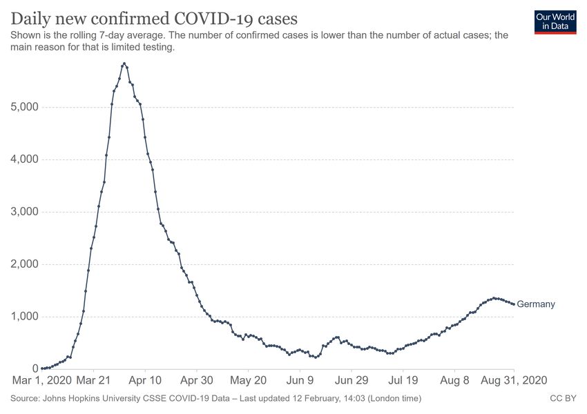
The most related papers to ours are from Betcherman et al. (2020) and from Juranek et al.
(2020). The first paper uses a difference-in-difference approach to assess the impact of a
layoff restriction intervention and finds that especially hampered hiring is causing the in-
crease in unemployment in Greece, the second paper evaluates different policy styles in a
cross-country study of Scandinavia and finds that Sweden only faced a minor labor market
reaction. Bauer and Weber (2020) examined the effects of the containment measures on the
job-finding and separation rate, however, the data was very limited at that point of time. In
comparison to these papers, our uses comprehensive data and allows for a thorough research
design, e.g. better control of time-invariant differences across region using panel regressions.
Furthermore this paper allows to better disentangle the effects of length and strength of the
lockdown.

The findings are the following: For the length of the lockdown we find that an additional day
of closure lead to an increase in the separation rate of 2.7 percent and a decrease in the job-
finding rate of 1.8 percent. For the strength of the lockdown the results show that a higher
the degree of closure, increase separations and lower job findings to a similar extent.

In a back-of-the-envelope calculation, we find that 31 percent of the considerably increased
inflows from employment into unemployment, and 33 percent of the reduced outflows from
unemployment to employment in the first wave were due to the treatment effect of the lock-
down measures. This increased unemployment in the short run by 80,000 persons.

In general, economic closures impact unemployment flows and short-time work more strongly
than curfews. Both, separations and job findings are affected. We find non-linearities in the
regressions, which point to two facts. First, further days of closure are less important once
the lockdown already started. Second, the lasting hiring weakness after the lockdown is not
specific to lockdown sectors.

While Section 2 presents some facts about the events during the Covid-19 pandemic in Ger-
many, section 3 and 4 display our regression exercise. Section 5 is highlighting the effects on
short-time work. Section 6 provides robustness checks. Section 7 concludes.

2 Germany in the first wave of the
pandemic

On January 27th 2020 the first infection with the Covid-19 virus was detected in Germany.
Initially, the pubic authorities kept the spread of the virus under control by tracking the in-

IAB-Discussion Paper 10|2021 8

fection chain. Nonetheless, in February and March, the infection numbers started to increase
rapidly (see Figure 1). In mid march, the German government decided to take action. A lock-
down was imposed from mid March to mid April. Travel was restricted, schools and child care
were closed, and also retail.

Figure 1: Daily number of confirmed cases over time

Source: COVID-19 Data Repository by the Center for Systems Science and Engineering (CSSE) at Johns Hopkins
University.

While this policy was effective in reducing the infection numbers, it also caused distortions
in the economy (e.g., Weber, 2020). In April and May, the numbers of notifications for short-
time work, the German job retention scheme, rocketed. But also unemployment increased
severely. Figure 2 shows both outcomes.

Over the summer, the situation relaxed. Short-time work and unemployment started to de-
crease, though did not reach the pre-recession level. In fall, the rate of infection started to
increase again, and a second lockdown followed. While the effect on the infections can be
easily tracked in real time. The reaction on the labour market is still ongoing and will be re-
vealed with a time delay. As it will take time to vaccinate the population because vaccine is
limited, there is a possibility, that we will have to have a lockdown every now and then.

In the light of these considerations, the question that naturally arises as labor economist is
which effects the strength and the length of a lockdown exhibits in terms of labor market
outcomes. Looking at data of the first lockdown and the subsequent recovery, we shed some
light on both dimensions. Furthermore, we are interested in which channel is driving the un-
employment result, namely separations and job-findings. Figure 3 shows the separation and
job-finding rate over time. It becomes evident that the separation rate quickly normalised
after a strong hike, but the job finding rate remained subdued to a considerable extent.

IAB-Discussion Paper 10|2021 9

Figure 2: Persons in notifications of short-time work and unemployment over time.

Source: Statistics of the Federal Employment Agency.

Besides the ins and outs, there are further flows forming the unemployment pool. However,
we neglect them in this paper though they are hit by the pandemic as well. These flows are
flows from unemployment to measures of active labor market policy and vice versa, and flows
from and to out-of-the-labor-force. For instance, in the first wave of the pandemic further
training and other measures of active labor market policy were suspended, which also caused
unemployment to rise.

3 Impact Channel: Lockdown length

In this section we want to understand how the length of a lockdown contributes to the rise in
the unemployment stock by taking a closer look at the job finding and the separation chan-
nel. We use administrative data combined with an innovative data set (see Bauer and Weber,
2020), that keeps track of the course of the measures across regions and time1 .

As dependent variables we use the flows between employment and unemployment for 156
Employment Agency districts. We consider the change in the seasonally adjusted separation

1
 This novel data set includes not just curfews and economic closure, but school closure. The data set is up-
dated regularly and publicly available. See http://doku.iab.de/arbeitsmarktdaten/data_corona_measures.xlsx

IAB-Discussion Paper 10|2021 10

Figure 3: Separation rate (left axis) and job-finding rate (right axis) across time.

 .09
 .01

 .08
 .009

 job-finding rate
separation rate

 .07
 .008

 .06
 .007

 .05
 .006

 0 2 4 6 8
 time

 sep_mean jfr_mean

Source: Statistics of the Federal Employment Agency. Own calculations.

and job finding rate from February to August 2020. The former is computed by taking the
inflows from employment to unemployment divided by the stock of employment, the latter is
determined by taking the outflows from unemployment to employment divided by the stock
of unemployment. The flows and stocks are administrative data of the Federal Employment
Agency and are counted in between to cutoff dates, where the cutoff date lies in the middle
of a month. For instance, for the month of April, the data is measured between the 13th of
March and the 14th of April. This is especially important, as the first official governmental
reaction regarding Covid-19 was decided on the 12th of March and was implemented on the
13th of March in the federal states. Hence we are confident that our data tracks the evolution
of the labor market aggregates, especially between March and April, very detailed.

As explanatory variables we use the days of economic closures and days of curfews. These
were determined via comprehensive research and compiled in a dataset. We calculate the
days of closure and curfews for a particular month by using the exact same cutoff date as
in the administrative data. For the data in April, that means the number of days reflect how
early the measures came into force regionally (because all measures persisted at least un-
til mid April). Over time it displays how log the lockdown in one agency district persisted
in comparison to another. The measures in the Employment Agency districts vary mainly
because districts belong to different federal states, but in some districts certain special mea-
sures exist. The data on closures were researched for the sectors of retail, accommodation,
restaurants, bars/clubs, cinemas, trade fairs/large-scale events, smaller events, other educa-
tion, art/entertainment/recreation and hairdressers/cosmetics, and combined into one clo-
sure variable per district by averaging.

IAB-Discussion Paper 10|2021 11

Figures 4 and 5 show the two variables over time and aggregated at the level of the federal
states. Though one might expect that there are more cautious states or districts which might
directly transforms into more economic closure days and curfews at the same time, Figure
5 shows that this appears not to be the case in Germany. A higher number of curfews is not
automatically connected with a high number of economic closures. Furthermore, because
the infection rate in the economy declined over time, the number of days of the measures is
decreasing over time as well. The figures depict the relative numbers of days. In absolute
terms, considering the 156 districts, there are on average 15 closing days (standard deviation
of 10) across the period under consideration. The average for the days of curfews is 27 days
(standard deviation of 6).

Figure 4: Average number of days of economic closures and curfews over time
 1
 .8.6
percent
 .4
 .2
 0

 4 5 6 7 8

 mean of economic closures mean of curfews

Note: Figure 4 shows the days of economic closure and curfews relative to the total days of the certain month
for each month beginning in April.
Source: own calculations.

We run fixed effects regression, weighted by the stock of employment to account for the dis-
trict size. This implies that the industry composition, the labor market status before the crisis,
and the regional differences are controlled for. Further we include the regional COVID-19 in-
fection rate at the cutoff date of the respective month. Several states never terminated the
curfew but instead changed the mode of the curfew, for instance, they allowed people from
one household to meet with another households. To control for potential bias in the curfew
variable, we add a variable that collects the number of days per month, in which people from
two different households can meet. Furthermore we include autoregressive parameters up
to lag 2. This controls for any persistence of the outcome variables. The regression equation
reads as follows:

IAB-Discussion Paper 10|2021 12

Figure 5: Average number of days of economic closures and curfews across federal states
1
.8
.6
.4
.2
0

 Baden Wuerttemberg

 Bavaria

 Berlin

 Brandenburg

 Bremen

 Hamburg

 Hesse

 Mecklenburg-Western Pomerania

 Lower Saxony

 North Rhine-Westphalia

 Rhineland-Palatinate

 Saarland

 Saxony

 Saxony-Anhalt

 Schleswig-Holstein

 Thuringia
 mean of economic closures mean of curfews

Note: Figure 5 shows the days of economic closure and curfews relative to the total days of the certain month
for each federal state.
Source: own calculations.

flow rate = 0 + 1 curfew + 2 economic closure + controls + (3.1)

The regression results in Table 1 shows, that the economic closures have an effect of +0.0152
on the separation rate, which means that one more closing day raises the regional separation
rate by 1.52 percent. On top, an additional day of curfew leads to an increase in the separation
rate by 0.13 percent. On the job-finding rate, the variable of economic closures has an effect
of -0.0106, i.e. another closing day leads to a 1.06 percent lower job-finding rate. Curfews
decrease the job-finding rate by 0.61 percent. Both channels operating via separations and
new hires are relevant. While curfews appear to have a reaction of similar size, economic
closures appear to have a stronger effect on the separation margin.

As the days of closure and the curfews are hump-shaped over time, we also added nonlin-
earities, that drive our results. This is our preferred regression. We find that adding squared
terms of the variables on economic closures and curfews initially strengthens the effect: for
the separation rate we find an increase of 2.7 percent, and for the job-finding rate a decrease

IAB-Discussion Paper 10|2021 13

Table 1: Regression of labour market flows on closing days - Robustness Check

 Dependent variable log(Separation rate) log(Job-finding rate)
 Economic closures 0.0152 0.02743 −0.0106 −0.0177
 (15.64) (8.42) (−10.41) (−4.10)
 Economic closures (squared) −0.0005 0.0006
 (−3.77) (3.20)
 Curfew 0.0013 0.0186 −0.0061 −0.0111
 (2.23) (8.49) (−5.18) (−3.19)
 Curfew (squared) −0.0006 0.0003
 (−7.90) (2.38)

Note: T-values in parenthesis. Robust (Huber/White) standard errors. Regression weighted by stock of employ-
ment.
Source: Statistics of the Federal Employment Agency, own calculations.

of 1.8 percent. Furthermore, the effects are not constant over time. In Figure 6 we show how
the effects evolve over a certain time horizon (upper panel), and that the marginal effect of
another day of closure (which is given by the first derivative) is decreasing over time for sep-
arations, and increasing over time for job-findings (see lower panel).

IAB-Discussion Paper 10|2021 14

Figure 6: Total and marginal effects of economic closures (solid lines) and curfews (dotted line) on
separation rate (upper panel) and job-finding rate (lower panel)

Note: Own calculations.

IAB-Discussion Paper 10|2021 15

4 Impact Channel: Lockdown strength

In this section we make use of job findings and separations (in levels) across industry sectors
(NACE Rev. 2, 2-digit) for the 16 federal states in Germany. We deviate here from the regional
classification used in section 4 because of data availability. Furthermore, we cannot compute
a job finding rate, as unemployment by industry sector is nonexistent.

We use a difference-in-difference approach, distinguishing industries that are treated by the
economic closures from the other industries. We use a special application of this approach
by replacing the binary treatment by the ”bite”. We borrow this procedure from the literature
that is concerned with the measurement of the effects of a nationwide minimum wage on em-
ployment (see, for instance, Card(1992) or a recent application from Caliendo et al. (2018)).
We use a variable that is bounded between 0 and 1 and indicates to which degree an industry
sector was closed in the lockdown between mid March and April. For sectors that were closed
by decree and are an enclosed sector in the NACE Rev. 2 classification, we assume a closure
of 100 percent. Those sector are, for instance, the travel sector and services in recreation and
sports. Also the automobile industry2 closed fully.

For sectors that were not fully closed by decree but faced some exemptions or in cases where
sectors were closed that are smaller than the category in the NACE Rev. 2 classifications we
assume a degree of closure by relying on several statistics, such as data on the sales volume,
sector size within the 2-digit category, productive share and demand projections. This pro-
vides the following assumptions: For ”Wholesale and retail trade and repair of motor vehicles
and motorcycles” we set the closure to 50 percent, approximating the share of trade while
garages were still operating. Accommodation and Food and beverage service activities is one
industry in our classification, and, because restaurants were allowed to offer take-away ser-
vice, we assume a closure of this industry of 80 percent, which is based on the loss in sales
volume according to the Federal Statistical Office. For wholesale and retail we assumed 40.5
percent, as groceries, pharmacies, drug stores and gas stations, which already make up 50
percent in terms of the productive share, were still running during lockdown and faced an
increase in demand. For land transport and transport via pipelines we set the rate to 32.8
percent, which stands for the majority of passenger services which also faced a decrease in
demand of about 20 percent. Libraries, archives, museums and other cultural activities, Cre-
ative arts and entertainment activities and Gambling and betting activities in sum are closed
to 70 percent, because most of the industries were closed by decree, except gambling. Other
personal service activities is assumed to be closed about 58 percent which corresponds to
the share of beauty treatments and hair dressers within the industry. Below 20 percent of clo-

2
 While the automobile industry was not closed by decree, because of its factural shutdown we take it as
treated (just as parts of transport.)

IAB-Discussion Paper 10|2021 16

sure was given to the industries of Education (standing for education beyond the schooling
system), Security and investigation, Services to buildings and landscape, office support and
other business support activities (which approximates the share of exhibition stand construc-
tion which is situated within that sector), Motion picture, video and television programme
production, sound recording and music publishing activities (corresponding to the produc-
tion share of cinemas).

We use random effect models and control for a comprehensive set of variables which stem
from the Establishment History Panel (BHP)(see Ganzer et al. (2020) for a full description of
the data set). The BHP is a cross sectional dataset that contains all the establishments in
Germany which are covered by the IAB Employment History (BeH) 3 and have at least one
employee liable to social security. We use the BHP to add information on the average share
of certain worker groups in the establishments operating in the industries in the regions, in-
formation about the average wage structure and the age of the establishments. Furthermore,
we control for the infection rate at the cutoff date of the respective month.

Our estimation equation reads as follows:

 ( ) = 0 + 1 ℎ + 2 + 3 ℎ × + + , (4.1)

where ( ) holds the logged separations or hirings in region , industry and time 
(March to August 2020). ℎ is a time dummy that takes on the value of 1 in the respective
month. As first closure measures came into force on March 13th, and the inflows in April are
measured between 13th of March and 14th of April, the April dummy is the first point in time
after lockdown. The reference date is March. The variable is bounded between 0 and
1, showing the degree of closure of an industry during lockdown and is time-invariant. The
logic is the following: On the one hand the degree of economic closures during the lockdown
has a direct effect on the flows in April, but it might also be the case that the effects spills over
to the proceeding months. We check this by assessing a treatment effect for each month from
April to August. This treatment effects are given by the interaction term of ℎ and 
with coefficient 3 . This interaction measures the strength of the treatment effect because of
the closure measures due to COVID-19. holds the control variables with coefficient vector
 , and is an industry-region-time specific error term.

Table 2 shows the effects of interest. A change in the degree of closure (from 0 to 1, i.e. 100 per-
cent) increases separations across industry and region by initially 46 percent and decreases
job-findings by 46 percent. This effect vanishes out over the following months. While for sepa-

3
 For more information follow this link.

IAB-Discussion Paper 10|2021 17

rations the effect persists until July, for the job-findings the effects already vanish in June (sta-
tistically insignificant) 4 . A back-of-the-envelope calculation in which we multiply the mean
degree of economic closure in the total economy with the (significant) coefficient of the in-
teraction terms, and sum over time, we end up with an average total effect on separations of
roughly 11 percent and on job findings of -12 percent. This implies that while the job finding
rate remained subdued also after the end of the lockdown (Figure 3), this was a broader effect
of the general crisis and no causal effect confined to the lockdown sectors.

Table 2: Regression of separations and hirings on degree of closure

 log(separations) log(hirings)
 treatment 0.5010 0.5668
 (2.86) (2.98)
 time
 April 0.2012 −0.3245
 (13.00) (−18.68)
 May 0.1412 −0.3050
 (7.55) (−14.15)
 June 0.0465 −0.0002
 (2.42) (−0.01)
 July −0.0211 −0.0751
 (−1.07) (−3.23)
 August −0.0492 0.0086
 (−2.33) (0.34)
 time × treatment
 April 0.4643 −0.4620
 (9.26) (−8.62)
 May 0.2030 −0.5416
 (4.20) (−10.72)
 June 0.1179 0.0512
 (2.55) (0.80)
 July 0.1168 0.0892
 (2.39) (1.89)
 August 0.0439 −0.0036
 (1.06) (−0.07)
Note: T-values in parentheses.
Source: Statistics of the Federal Employment History; Establishment History Panel 2018, own calculations.
©IAB

4
 As the closure variable is bounded between 0 and 1, expansion bias might exist (see Rigobon and Stoker,
2007)

IAB-Discussion Paper 10|2021 18

5 Short-time work

In Germany - just as in many other countries - the labour market was shielded from the crisis
effects by job retention schemes at large scale. Hence, in this section, we apply our regres-
sion framework to notifications for short-time work (see figure 2). Each firm has to apply
for short-time work, and indicate how many workers will be covered by this job retention
scheme. If firms are eligible, they will send their employees in short-time work, which will re-
ceive compensation from the Federal Employment Agency. We devide the number of persons
in short-time work by the number of employees in the respective month and in the respective
Employment Agency district. This leaves us with a short-time work rate, which we then log.
Running regressions in the same spirit as in section 4 provides the following results.

Table 3: Regression of persons in short-time work on closing days and curfews

 log(rate of short-time workers)
 Economic closures 0.0556
 (21.13)
 Curfews 0.0051
 (1.75)
Note: T-values in parentheses. The time series starts in January. Additional controls: Dummy indicating when
it was allowed to meet persons of more than one household, the rate of infection at the cutoff date.
Source: Statistics of the Federal Employment History; Establishment History Panel 2018, own calculations.
©IAB

Table 3 shows that economic closures have stronger effects on the share of short-time work
than curfews. While economic closure increase the rate of short-time work by roughly 6 per-
cent, curfews increase it by 0.5 percent.

Because the number of workers in short-time work reacted earlier as unemployment, we start
with the treatment period earlier than in the regressions above. Table 8 shows that the initial
impact of the lockdown was high, but that the effect gets smaller over time. For non-treated
industries (sectors not directly affected by closures), the effect starts at an increase of short-
time work of 243 percent in March and for treated sectors (sectors with a certain degree of
closure) the short-time work increased by even 400 percent. That implies, that the industry
sectors that were hit hardest in terms of closure, used a lot more short-time work, namely 400
percent more than not directly affected industries.

IAB-Discussion Paper 10|2021 19

Table 4: Regression of persons in short-time work on degree of closure

 log(persons in short-time work)
 treatment −2.6537
 (−8.03)
 time
 March 2.4302
 (26.85)
 April 3.2531
 (28.31)
 May 3.1979
 (24.80))
 June 2.9208
 (21.66)
 July 2.5772
 (18.63)
 time × treatment
 March 4.0405
 (11.17)
 April 3.8110
 (11.10)
 May 3.6234
 (10.67)
 June 3.5157
 (10.44)
 July 3.4342
 (9.95)
Note: T-values in parentheses.
Source: Statistics of the Federal Employment History; Establishment History Panel 2018, own calculations.
©IAB

IAB-Discussion Paper 10|2021 20

6 Robustness

6.1 Robustness on length

We further checked to which extent the lockdown shows prolongated effects by controlling
for lags. Table 6shows that this procedure gives results that lie between the basic version and
the non-linear version but has a lot of insignificant effects.

Table 5: Regression of labour market flows on closing days - Robustness Check

 Dependent variable log(Separation rate) log(Job-finding rate)
 Economic closures 0.0109 −0.0127
 (7.58) (−6.48)
 Economic closures (lagged) 0.0113 −0.0024
 (10.48) (−1.83)
 Curfew 0.0019 0.0000
 (1.70) (0.00)
 Curfew (lagged) 0.0041 −0.0053
 (0.28) (−2.88)

Note: T-values in parenthesis. Robust (Huber/White) standard errors. Regression weighted by stock of employ-
ment.
Source: Statistics of the Federal Employment Agency, own calculations.

IAB-Discussion Paper 10|2021 21

6.2 Robustness on strength

In the main regression we used an estimate of degree of closure. In this robustness check
we consider two alternatives: First, we replace the degree of closure by a dummy variable.
This allows to estimate a classical diff-in-diff. Second, we instead use the share of the gross
value added affected by the closures in the industries that were not directly treated. The logic
behind is the following: While some industries are closed per decree, others were hit by these
measures through their linkages to the closed industries. To account for the full extent, we
generate the change in the gross value added of every industry caused by the closures via
their linkages in an input-output table. A full list of the degrees of closure and the loss in
value added including input-output linkages is given in the appendix.

Table 6: Regression of separations and hirings on degree of closure using input-output linkage
 Dummy variable loss in gross value added
 log(separations) log(hirings) log(separations) log(hirings)
 treatment 0.8350 0.8606 0.5848 0.6121
 (7.44) (7.66) (3.51) (3.43)
 time
 April 0.1985 -0.3294 0.1786 -0.3005
 (12.48) (-18.38) (11.10) (-15.33)
 May 0.1406 -0.3190 0.1329 -0.2735
 (7.30) (-14.43) (7.02) (-11.88)
 June 0.0494 -0.0008 0.0443 0.0092
 (2.50) (-0.03) (2.22) (0.38)
 July -0.0090 -0.0813 -0.0269 -0.0739
 (-0.45) (-3.43) (-1.30) (-2.94)
 August -0.0475 0.0013 -0.0491 0.01273
 (-2.20) (0.05) (-2.25) (0.48)
 time × treatment
 April 0.2758 -0.2366 0.4447 -0.4487
 (10.04) (-8.08) (12.37) (-10.11)
 May 0.1148 -0.2429 0.1859 -0.5421
 (4.68) (-7.45) (5.17) (-12.21)
 June 0.0506 0.0325 0.0941 -0.0127
 (2.20) (1.10) (2.62) (-0.28)
 July 0.0114 0.0768 0.1120 0.0564
 (0.43) (3.33) (3.11) (1.27)
 August 0.01257 0.0295 0.0302 -0.0238
 (0.55) (1.14) (0.84) (-0.54)

Note: T-values in parentheses.
Source: Statistics of the Federal Employment History; Establishment History Panel 2018, own calculations.
©IAB

IAB-Discussion Paper 10|2021 22

6.2.1 Timing of events

In the main regression we decided to use March as the reference month. This procedure al-
lows us to appropriately determine the effect of the closure measure by reducing the omitted
variable bias via controlling for the regional infection rate, which is not filled before March.
However, in this robustness check we performed a regression where we set the pre-crisis pe-
riod to January instead of March (i.e. assume an infection rate of zero before March). This
leaves us with results that are very similar in size and significance. Most importantly, it shows
that the treatment effects in February and March are negligible and insignificant. Accordingly,
March appears to be a proper reference month.5 See Table 8 in the Appendix for the results.

6.2.2 Back-of-the-envelope calculations

In order to assess the explanatory power of the regression results in Table 6, we run the fol-
lowing computations: First we assess how many more separations and less job-findings exist
by applying the coefficients of the treatment effects between April and August to the mean
level of separations and job findings between January and March and multiply this expres-
sion which the loss in output. Then we sum these additional separations and job findings
over time which gives us a cumulative treatment effect in both variables. Second we calculate
the cumulative increase in separations and job findings in our data accordingly and compare
these numbers. We can explain about 31 percent of the increase in separations, and about
33 percent of the reduction in job findings. Overall, this stands for 80 thousand more people
in unemployment.

Note that this does not equal the total number of additional separations (or lost hirings) in
the affected sectors: The treatment effect measures only the part that exceeds the effect all
sectors were subject to. I.e., a substantial part of the labour market reaction was not directly
due to domestic containment measures, but due to other general crisis effects. Candidates
are increased uncertainty, worsened expectations, supply chain problems and reductions in
export demand.

5
 Note that we also visually inspected the common trend assumption in the binary case, which shows no
abnormality.

IAB-Discussion Paper 10|2021 23

7 Conclusion

We find that in Germany, especially the separations increased through the containment mea-
sures. While the length of the lockdown was identified in an innovative data set that tracks
the number of days of economic closure and curfew, the strength of the lockdown was given
by the estimated degree of closure mainly based on national statistics on sales and industry
share of industries hit.

For the length of the lockdown we find that an additional day of closure lead to an increase
in the separation rate of 2.7 percent and a decrease in the job-finding rate of 1.8 percent.
For the strength of the lockdown the results show that a higher degree of closure, increase
separations and lower job findings to a similar extent. In both dimensions, we find that the
effects are non-linear over time.

For the effects of the lockdown length, the non-linearities shed light on the question, whether
an additional day of lockdown is more painful or not. We find that further days are less im-
portant once the lockdown already started. A possible explanation might be that economic
agents learn to deal with the situation.

The nonlinearities in the strength regression, show that the additional effects of the spring
lockdown quickly taper off. While Figure 3 shows that the separation rate indeed normalised,
this does not hold for the job finding rate. However, the fact that job findings remained sub-
dued also after the end of the lockdown has been a broader effect of the general crisis and no
causal effect confined to the lockdown sectors.

For short-time work, we find a significant impact for the length of economic closures and cur-
few. The effect of economic closures on short-time work is ten times stronger than the effect
of the curfews. For the strength of the measures, we also find clear significant effects. In-
dustries that are particularly hit by the crisis use short-time work considerably oftener. Again
these effects are non-linear over time.

In a nutshell, economic closures impact unemployment flows and the number of short-time
workers more strongly than curfews. Both, separations and job findings are affected. The
lasting hiring weakness after the lockdown is not specific to lockdown sectors. In a back-
of-the-envelope calculation, we find that 31 percent of the considerably increased inflows
from employment into unemployment, and 33 percent of the reduced outflows from unem-
ployment to employment in the first wave were due to the treatment effect of the lockdown
measures. This increased unemployment in the short run by 80,000 persons.

IAB-Discussion Paper 10|2021 24

When assessing these results, two points should be kept in mind: First, the available data
measure effects up to August. Secondly, we consider immediate effects in the first wave.
These are probably not applicable to the second wave as there are learning effects for the
firms and a more positive perspective due to progressive vaccinations. Without the mea-
sures, however, an uncontrolled spread of the virus could possibly have caused much greater
damage in the medium run.

Notwithstanding, our results show which opportunity costs of the containment measures and
their length and strength have to be taken into account by policy makers.

IAB-Discussion Paper 10|2021 25

References
 Bauer, Anja; Weber, Enzo (2020): COVID-19: how much unemployment was caused by
 the shutdown in Germany?. Applied Economics Letters (2020), p. 1-6.

 Betcherman, G.; Giannakopoulos, N.; Laliotis, I.; Pantelaiou, I.; Testaverde, M.; Tzimas, G.
 (2020): Reacting quickly and protecting jobs: The short-term impacts of the COVID-19
 lockdown on the Greek labor market.

 Bradley, Jake; Ruggieri, Alessandro; Spencer, Adam (2020): Twin peaks: Covid-19 and
 the labor market. No. 2020/06. 2020.

 Birinci, Serdar (2020): Unemployment Insurance and Vulnerable Households During the
 COVID-19 Pandemic. Available at SSRN 3612309.

 Caliendo, Marco; Fedorets, Alexandra; Preuss, Malte; Schröder, Carsten; Wittbrodt, Linda
 (2018): The short-run employment effects of the German minimum wage reform.
 Labour Economics, Volume 53, p. 46-62.

 Card, David (1992): Using regional variation in wages to measure the effects of the federal
 minimumwage. Industrial and Labor Relations Review, 46(1), p. 22-37.

 Ganzer, Andreas; Schmidtlein, Lisa; Stegmaier,Jens; Wolter, Stefanie (2020): Establish-
 ment History Panel 1975-2018. FDZ-Datenreport, 01/2020 (en), Nuremberg.
 DOI: 10.5164/IAB.FDZD.2001.en.v1

 Juranek, S.; Paetzold, J.; Winner, H.; Zoutman, F. (2020): Labor market effects of COVID-
 19 in Sweden and its neighbors: Evidence from novel administrative data. NHH Dept.
 of Business and Management Science Discussion Paper, (2020/8).

 Kapicka, Marek; Rupert, Peter (2020): Labor markets during pandemics. Manuscript, UC
 Santa Barbara.

 Rigobon, Roberto; Stoker, Thomas (2007): Estimation with censored regressors: Basic
 issues. International Economic Review, 48.4, p. 1441-1467.

 Sazmaz, Elif Beyza; Ozkok, Emine Irem; Simsek, Huseyin; Gulseven, Osman (2020): The
 Impact of COVID-19 on European Unemployment and Labor Market Slack (January
 14, 2021). Available at SSRN: https://ssrn.com/abstract=3766376.

 Tetlow, Gemma; Pope, Thomas; Dalton, Grant (2020): Coronavirus and unemployment:
 the importance of government policy: a five nation comparison, 30 p..

 Weber, Enzo (2020): Which measures flattened the curve in Germany? Covid economics,
 No. 24, p. 205-217.

IAB-Discussion Paper 10|2021 26

Appendix

8 Input-Output Linkage

Table 7: Inflows to unemployment from employment subject to social security contributions

 loss of value degree of clo-
 Code ”Classification of Products by Activity”
 added sure
 01 Crop and animal production, hunting and related service activities -0,0064 0,0000
 02 Forestry and logging -0,0030 0,0000
 03 Fishing and aquaculture -0,1151 0,0000
 05 Mining of coal and lignite 0,0000 0,0000
 06 Extraction of crude petroleum and natural gas -0,0070 0,0000
 07-09 Mining and quarrying and mining support service -0,0005 0,0000
 10-12 Manufacture of food products, beverages, tobacco -0,0425 0,0000
 13-15 Manufacture of textiles and wearing apparel -0,0227 0,0000
 16 Manufacture of leather, wood and cork -0,0357 0,0000
 17 Manufacture of paper and paper products -0,0303 0,0000
 18 Printing and reproduction of recorded media -0,0995 0,0000
 19 Manufacture of coke and refined petroleum products -0,0507 0,0000
 20 Manufacture of chemicals and chemical products -0,0109 0,0000
 Manufacture of basic pharmaceutical products and pharmaceuti-
 21 0,0000 0,0000
 cal preparations
 22 Manufacture of rubber and plastic products -0,1371 0,0000
 23 Manufacture of other non-metallic mineral products -0,0388 0,0000
 24 Manufacture of basic metals -0,1872 0,0000
 Manufacture of fabricated metal products, except machinery and
 25 -0,1089 0,0000
 equipment
 26 Manufacture of computer, electronic and optical products -0,0067 0,0000
 27 Manufacture of electrical equipment -0,0353 0,0000
 28 Manufacture of machinery and equipment n.e.c. -0,0171 0,0000
 29 Manufacture of motor vehicles, trailers and semi-trailers -1,0000 1,0000
 30 Manufacture of other transport equipment -0,0058 0,0000
 31-32 Manufacture of furniture and Other manufacturing -0,0008 0,0000
 33 Repair and installation of machinery and equipment -0,1089 0,0000
 35 Electricity, gas, steam and air conditioning supply -0,0609 0,0000
 36 Water collection, treatment and supply -0,0698 0,0000
 37-39 Sewerage, Waste collection, disposal and remediation activities -0,0524 0,0000
 41 Construction of buildings -0,0021 0,0000
 42 Civil engineering -0,0118 0,0000
 43 Specialised construction activities -0,0314 0,0000
 Wholesale and retail trade and repair of motor vehicles and motor-
 45 -0,7545 0,5000
 cycles
 46 Wholesale trade, except of motor vehicles and motorcycles -0,4581 0,4050

IAB-Discussion Paper 10|2021 27

loss of value degree of clo-
 Code ”Classification of Products by Activity”
 added sure
 47 Retail trade, except of motor vehicles and motorcycles -0,4453 0,4050
 49 Land transport and transport via pipelines -0,5316 0,3280
 50 Water transport -0,0231 0,0000
 51 Air transport -0,9222 0,7500
 52 Warehousing and support activities for transportation -0,6988 0,5000
 53 Postal and courier activities -0,2115 0,0000
 55-56 Accommodation and Food and beverage service activities -0,8231 0,8000
 58 Publishing activities -0,0503 0,0000
 Motion picture, video and television programme production and
 59-60 -0,0249 1,0000
 Programming and broadcasting activities
 61 Telecommunications -0,0643 0,0000
 Computer programming, consultancy and related activities and In-
 62-63 -0,0528 0,0000
 formation service activities
 64 Financial service activities, except insurance and pension funding -0,0493 0,0000
 Insurance, reinsurance and pension funding, except compulsory
 65 -0,0471 0,0000
 social security
 66 Activities auxiliary to financial services and insurance activities 0,0000 0,0000
 68 Real estate activities -0,0580 0,0000
 Legal and accounting activities and Activities of head offices; man-
 69-70 -0,0711 0,0000
 agement consultancy activities
 Architectural and engineering activities; technical testing and anal-
 71 -0,0457 0,0000
 ysis
 72 Scientific research and development 0,0000 0,0000
 73 Advertising and market research -0,1372 0,0000
 Other professional, scientific and technical activities and Veteri-
 74-75 -0,0790 0,0000
 nary activities
 77 Rental and leasing activities -0,0913 0,0000
 78 Employment activities -0,1606 0,0000
 Travel agency, tour operator and other reservation service and re-
 79 -1,0000 1,0000
 lated activities
 Security and investigation, Services to buildings and landscape, of-
 80-82 -0, 7670 0,1600
 fice support and other business support activities
 84 Public administration and defence; compulsory social security -0,0114 0,0000
 85 Education -0,1399 0,1300
 86 Human health activities -0,0012 0,0000
 Residential care activities and Social work activities without ac-
 87-88 0,0000 0,0000
 commodation
 Entertainment activities, Libraries, archives, museums and Gam-
 90-92 -0,7180 0,7000
 bling
 93 Sports activities and amusement and recreation activities -1,0000 1,0000
 94 Activities of membership organisations -0,0335 0,0000
 95 Repair of computers and personal and household goods -0,0861 0,0000
 96 Other personal service activities -0,5967 0,5800
 Activities of households, goods- and services-producing activities
 97-98 0,0000 0,0000
 of private households for own use

Source: Federal Statistical Office. Own calculations.

IAB-Discussion Paper 10|2021 28

9 Timing of events

Table 8: Regression of separations and hirings on degree of closure - reference month January
 log(separations) log(hirings)
 treatment 0.5138 0.5346
 (2.91) (2.85)
 time
 February −0.0271 −0.0368
 (−3.01) (−3.34)
 March 0.0515 −0.0299
 (5.61) (−2.68)
 April 0.2604 −0.3698
 (23.59) (−24.89)
 May 0.2035 −0.3563
 (17.93) (−25.94)
 June 0.1098 −0.0536
 (9.62) (−3.82)
 July 0.0429 −0.1298
 (3.88) (−10.50)
 August 0.0160 −0.0484
 (1.45) (−3.63)
 time × treatment
 February 0.0050 0.0118
 (0.19) (0.39)
 March −0.0148 0.02286
 (−0.46) (0.71)
 April 0.4495 −0.4395
 (9.74) (−7.81)
 May 0.1882 −0.5193
 (4.38) (−9.67)
 June 0.1033 0.0734
 (2.21) (1.06)
 July 0.1022 0.114
 (2.16) (2.10)
 August 0.0293 0.0187
 (0.69) (0.32)
Note: T-values in parentheses.
Source: Statistics of the Federal Employment History; Establishment History Panel 2018, own calculations.
©IAB

IAB-Discussion Paper 10|2021 29

Imprint
IAB-Discussion Paper 10|2021

Publication Date
28 July 2021

Publisher
Institute for Employment Research
of the Federal Employment Agency
Regensburger Straße 104
90478 Nürnberg
Germany

All rights reserved
Reproduction and distribution in any form, also in parts, requires the permission of the IAB

Download
http://doku.iab.de/discussionpapers/2021/dp1021.pdf

All publications in the series “IAB-Discusssion Paper” can be downloaded from
https://www.iab.de/en/publikationen/discussionpaper.aspx

Website
www.iab.de/en

Corresponding author
Anja Bauer
+49 911 179-3366
E-Mail Anja.Bauer@iab.de

Enzo Weber
Enzo.Weber@iab.de