Health Analytics REPORT 04/2018
←
→
Page content transcription
If your browser does not render page correctly, please read the page content below
REPORT
                                                                                    04/2018

Health Analytics

Makhlysheva A., Budrionis A., Chomutare T., Nordsletta A.T., Bakkevoll P.A., Henriksen T.,
Hurley J.S., Bellika J.G., Blixgård H., Godtliebsen F., Skrøvseth S.O., Solvoll T., Linstad L.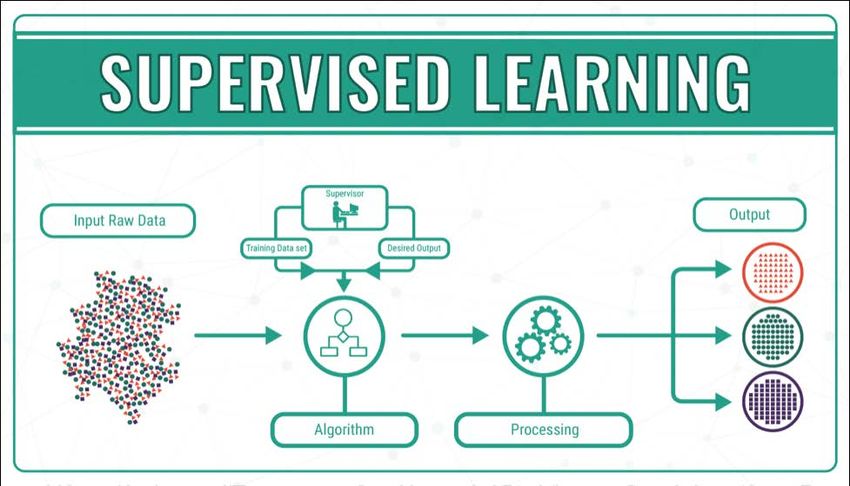
Health Analytics

Report number            Summary
04-2018                  The health analy�cs review focuses on machine
                         learning, natural language processing, data mining and
Project manager          process mining methods: their usefulness, use cases,
Per Atle Bakkevoll       tools and relatedness to Norwegian healthcare.

Authors                  The report aims to increase the audience’s beter
Alexandra Makhlysheva    understanding of health analy�cs and the methods to
Andrius Budrionis        be u�lized in improving the performance of healthcare.
Taridzo Chomutare        Keywords
Anne Torill Nordsleta    Health data, health analy�cs, ar�ficial intelligence, ma-
Per Atle Bakkevoll       chine learning, deep learning, data mining, process
Torje Henriksen          mining, natural language processing
Joseph Stephen Hurley
Johan Gustav Bellika     Publisher
Håvard Blixgård          Norwegian Centre for E-health Research
Fred Godtliebsen         PO box 35, NO-9038 Tromsø, Norway
Stein Olav Skrøvseth
Terje Solvoll            E-mail: mail@ehealthresearch.no
Line Linstad             Website: www.ehealthresearch.no

ISBN 978-82-8242-086-0

Date
11.06.2018

Number of pages 88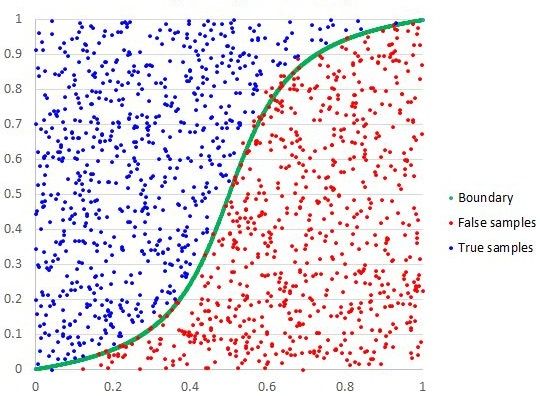
1

Table of contents
1.   Background........................................................................................................................... 4
     1.1. Project objec�ve ................................................................................................................... 5
     1.2. Approach ............................................................................................................................... 5
     1.3. Organiza�on of the report .................................................................................................... 5

2.   Machine learning .................................................................................................................. 6
     2.1. Defini�on of the concept ...................................................................................................... 6
     2.1.1     Supervised learning ....................................................................................................... 7
     2.1.2     Unsupervised learning ................................................................................................. 13
     2.1.3     Semi-supervised learning ............................................................................................ 16
     2.1.4     Reinforcement learning ............................................................................................... 17
     2.1.5     Neural networks .......................................................................................................... 18
     2.1.6     Interpretability of machine learning algorithms.......................................................... 21
     2.2. Usefulness – why do we need this technology? ................................................................. 22
     2.3. Status of the field ................................................................................................................ 23
     2.3.1     Reasons for ML rise...................................................................................................... 23
     2.3.2     Privacy concerns in machine learning ......................................................................... 25
     2.4. Use cases ............................................................................................................................. 26
     2.4.1     Diagnosis in medical imaging....................................................................................... 26
     2.4.2     Treatment queries and sugges�ons............................................................................. 27
     2.4.3     Drug discovery/drug development .............................................................................. 27
     2.4.4     Improved care for pa�ents with mul�ple diagnoses ................................................... 27
     2.4.5     Development of clinical pathways ............................................................................... 28
     2.4.6     Popula�on risk management ....................................................................................... 28
     2.4.6     Robo�c surgery ............................................................................................................ 28
     2.4.7     Personalized medicine (precision medicine) ............................................................... 29
     2.4.8     Automa�c treatment/recommenda�on...................................................................... 29
     2.4.9     Performance improvement ......................................................................................... 30
     2.5. How does this relate to Norway and the needs in Norwegian healthcare? ....................... 30

3.   Natural Language Processing (NLP) .......................................................................................32
     3.1. Defini�on of the concept .................................................................................................... 32
     3.1.1     Tasks NLP can be used for [110] ................................................................................. 33
     3.1.2     Example of NLP pipeline .............................................................................................. 33
     3.2. Usefulness – why do we need this technology? ................................................................. 34
     3.2. What is the knowledge in the field? ................................................................................... 35
     3.2.1     Seminal work ............................................................................................................... 35
     3.2.2     Current ac�vi�es and expected future trends ............................................................. 35
     3.3. Use cases ............................................................................................................................. 36
     3.3.1     Norway research and development cases ................................................................... 37
     3.4. How does NLP relate to the needs in Norwegian healthcare? ........................................... 37
     3.4.1     Elici�ng expert opinion using the Delphi Method ....................................................... 37
     3.4.2     Results from expert opinion survey ............................................................................. 38
     3.5. Tools and Resources ............................................................................................................ 39
     3.6. Acknowledgements............................................................................................................. 40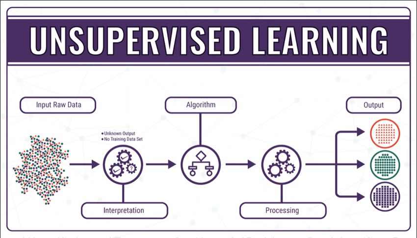
2
4. Knowledge discovery in databases (data mining and process mining) ....................................41
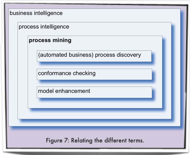
4.1. Defini�on of the concept .................................................................................................... 41
4.2. Usefulness – why do we need this technology? ................................................................. 45
4.3. What is the knowledge in the field? ................................................................................... 46
4.4. Use cases ............................................................................................................................. 47
4.5. How does this relate to Norway and the needs in Norwegian healthcare? ....................... 48
5. Tools ....................................................................................................................................49
5.1. Defini�on of the concept .................................................................................................... 49
5.2. Usefulness – Why do we need this? ................................................................................... 49
5.3. What is the knowledge in the field? ................................................................................... 50
5.3.1. Programming language ................................................................................................ 51
5.3.2. Scalability ..................................................................................................................... 51
5.3.3. Enterprise support ....................................................................................................... 51
5.3.4. Installa�on and ease of ge�ng started ....................................................................... 52
5.3.5. License ......................................................................................................................... 52
5.3.6. Impact on IT infrastructure .......................................................................................... 52
5.3.7. Interoperability between models ................................................................................ 52
5.3.8. Hardware dedicated to machine learning ................................................................... 53
5.4. Use cases ............................................................................................................................. 53
5.4.1. TensorFlow ................................................................................................................... 53
5.4.2. H2O.ai .......................................................................................................................... 54
5.4.3. Microso� Azure ........................................................................................................... 54
5.4.4. Gate Developer ............................................................................................................ 55
5.5. How does this relate to Norwegian healthcare? ................................................................ 56
6. Stakeholder mapping ...........................................................................................................58
6.1. Background, methodology, limita�ons and categoriza�on ................................................ 58
6.2. Norwegian stakeholders and ini�a�ves .............................................................................. 59
6.3. Swedish stakeholders .......................................................................................................... 67
7. Summary .............................................................................................................................70
References ..................................................................................................................................71
A. Publica�on sta�s�cs about machine learning in PubMed ......................................................82
Publica�on sta�s�cs ...................................................................................................................... 82
Main areas ..................................................................................................................................... 82
List of figures
Figure 1. Machine learning, other concepts, and their interconnec�ons in data science universe ....... 6
Figure 2. Supervised machine learning ................................................................................................... 7
Figure 3. Le�: Model performs poorly (underfi�ng). Center: Model generalizes well. Right: Model is
too complex and overfi�ng .................................................................................................................... 8
Figure 4. Bias and variance contribu�ng to total error ........................................................................... 8
Figure 5. Examples of classifica�on problems ......................................................................................... 9
Figure 6. Regression model example ....................................................................................................... 9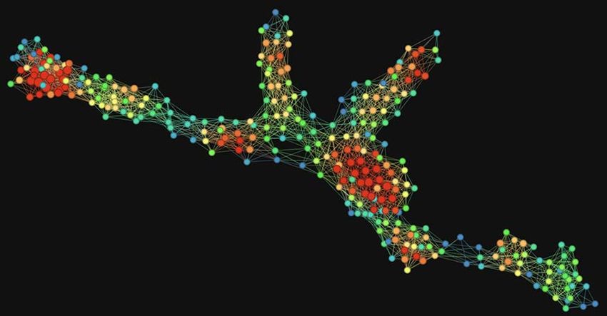
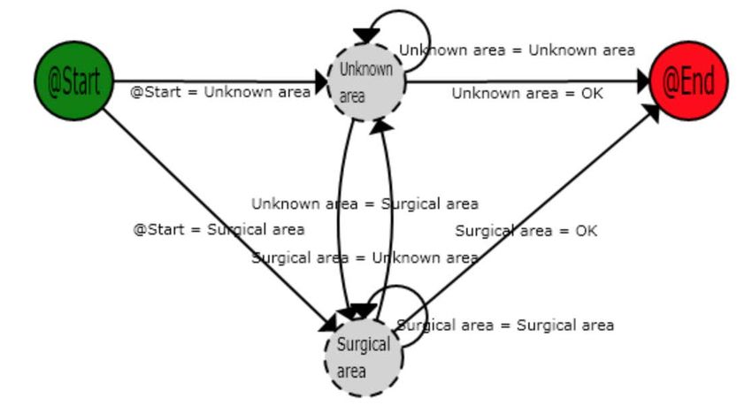
3

Figure 7. Logis�c regression example .................................................................................................... 10
Figure 8. An example of decision tree ................................................................................................... 10
Figure 9. Example of k-NN classifica�on................................................................................................ 11
Figure 10. An example of SVM work ..................................................................................................... 12
Figure 11. An example of how Random Forest algorithm works .......................................................... 12
Figure 12. An example of gradient boosted decision tree .................................................................... 13
Figure 13. Unsupervised machine learning ........................................................................................... 13
Figure 14. CT image segmenta�on (on the le� - original CT image, in the center - CT image using
threshold technique, on the right - edge-based Segmenta�on of CT image) ....................................... 14
Figure 15. An example of k-means clustering........................................................................................ 15
Figure 16. Three original variables (genes) are reduced to a lower number of two new variables
(principal components). Using PCA, the 2-D plane that op�mally describes the highest variance of the
data is iden�fied (le�). This 2-D subspace is then rotated and presented as a 2-D component space
(right)……………... .................................................................................................................................... 15
Figure 17. TDA visualiza�on of clinical and billing data from total knee replacement pa�ents ........... 16
Figure 18. Reinforcement machine learning ......................................................................................... 17
Figure 19. An example of neural network ............................................................................................. 18
Figure 20. Example of what each layer in CNN may learn based on face image dataset ...................... 19
Figure 21. Example of denoising autoencoder's work .......................................................................... 20
Figure 22. Example of recurrent neural network. The hidden layer forms a directed graph able to
feedback informa�on from previous calcula�ons ................................................................................. 20
Figure 23. Example of a basic deep belief network for binary classifica�on with k hidden layers ....... 21
Figure 24. Rela�onships among the technologies: ar�ficial intelligence (AI), machine learning (ML),
deep learning (DL) and natural language processing (NLP) .................................................................. 32
Figure 25. Finding structure in clinical text ........................................................................................... 34
Figure 26. Mitsuku chatlog .................................................................................................................... 36
Figure 27. Overview of steps in KDD ..................................................................................................... 42
Figure 28. An example of data dredging................................................................................................ 43
Figure 29. Process mining and its rela�on to other disciplines ............................................................. 43
Figure 30. An example process of pa�ent flow in surgical area in the hospital .................................... 45
4

1. Background
Demographic trends, availability of health personnel and new treatment methods challenge the sus-
tainability of healthcare. How can future health service be designed for more preven�ve, pa�ent-cen-
tered, and cost-effec�ve care, and reduce burden on health system? How can we u�lize ar�ficial intel-
ligence (AI) for providing equal accessibility and quality of health services to all ci�zens?
Health analy�cs is a process of deriving insights from health data to make informed healthcare deci-
sions. While such aspects of health analy�cs as the use of sta�s�cal models, data mining, and clinical
decision support have existed for decades, only recent availability of enormous volume of data from
various sources and increased processing power have made it readily available to support integrated
decision making. Machine learning, data and process mining and natural language processing are the
main topics in the report.
Data integra�on technologies provide completely new opportuni�es for advanced analy�cs. Health
analy�cs has evolved from being descrip�ve to being predic�ve and prescrip�ve.
       •    Descriptive analytics looks at what has already happened.
       •    Predictive analytics tries to say something about what is going to happen. This involves pro-
            jecting the trends and patterns in historical data and real-time data to predict, for example,
            the future development of health situation of a patient or patient groups in the population.
       •    Prescriptive analytics is a step further. By using medical knowledge, it can evaluate alterna-
            tive treatments and find the optimal one in a given situation. Prescriptive analytics is key in
            personalized medicine.
HIMSS 1 has developed a systema�c model, the Adop�on Model for Analy�cs Maturity 2 (AMAM),
used to evaluate maturity of healthcare organiza�ons within the analy�cs field. On the second most
advanced stage of the AMAM model, there are predic�ve analy�cs and risk stra�fica�on. Prescrip�ve
analy�cs and personalized medicine are on the most advanced stage; to get to this level, genomic
data must be available.
Good analyses require access to relevant high-quality data. A significant challenge for health data is
its heterogeneity and complexity. The healthcare processes generate a large amount of unstructured
data, such as medical images and free text. Therefore, in order to exploit the full poten�al of health
data, the machine-learning analy�cs tools can be u�lized. Moreover, for preserving the meaning of
data, it is necessary to harmonize it with both a common data format and terminology.
The governmental white paper “One Ci�zen - One Record” [1] promotes that “data should be availa-
ble for quality improvement, health monitoring, management and research”. The Norwegian e-health
strategy (2017-2022) [2] has “beter use of health data” as one of the strategic focus areas.
The Norwegian Directorate of e-health is developing a na�onal health analy�cs pla�orm, which will
“... simplify access to health data and facilitate advanced analy�cs across health registries, source
data, health records and other sources of health informa�on.” It is further stated: “The Directorate of
e-health aims to contribute to tes�ng and development of new technologies in health analy�cs, such
as ar�ficial intelligence, machine learning, algorithms and predic�ve analy�cs.” In addi�on, the Nor-
wegian Technological Council 3 has its own project focusing on AI and the welfare state [3].

1   htps://www.himss.org
2   htp://www.himssanaly�cs.org/amam
3The Norwegian Technological Council is an independent public body that provides advice to the Norwegian Parliament and the Norwegian
Government on new technologies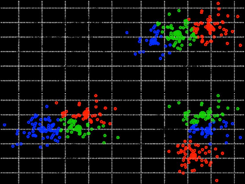
5

The implementa�on of large-scale e-health solu�ons challenges the organiza�on of health services,
including authority structures, financial systems, legal and ethical frameworks [4]. Research on the
implementa�on of na�onal large-scale solu�ons demonstrates this being a complex and �me-con-
suming task for the sector actors [5-7]. The establishment of the Na�onal Board for e-health and na-
�onal efforts to increase the sector’s capacity to implement will contribute to the dissemina�on of
knowledge to na�onal services [2].
Health analy�cs is a large and complex field. AI technology is gaining momentum in the development
of future digital services and tools for interac�on in healthcare. Therefore, it is important for
healthcare policymakers to acquire knowledge in this field.

The contribu�on of the report and the project is to improve awareness and increase knowledge and
skills about health analy�cs, ar�ficial intelligence and machine-learning techniques and how to u�lize
health analy�cs in improving the performance of healthcare.

Conduc�ng research and gathering informa�on for the report was performed as an exploratory litera-
ture study. Informa�on search has been done through PubMed, Google Scholar, and Google. In addi-
�on, interviews with the research groups and individual researchers were conducted. A web-based
survey was held among actors in natural language processing. To iden�fy relevant publica�ons and
stakeholders, the “snowball” sampling technique has been applied. By this method, exis�ng study
subjects recruit future subjects from their acquaintances.

The report chapters are machine learning, natural language processing, knowledge discovery in data-
bases, machine-learning tools, and stakeholder mapping. Several chapters include concept basics,
usefulness, and current knowledge in the field, use cases, and relatedness to the Norwegian
healthcare.
6

2. Machine learning
The applica�on of machine learning principles to health data can help find structure and extract
meaning from such data. Together with the vast amount and varia�on in data being produced about
people’s health, it is increasingly clear that machine learning in healthcare can contribute to improv-
ing both the efficiency and quality of medical care now and in the future.

The terms “ar�ficial intelligence” (AI) and “machine learning” (ML) are o�en used interchangeably.
However, they are not the same.
According to Merriam-Webster dictionary, artificial intelligence is “a branch of computer science
dealing with the simulation of intelligent behavior in computers”, and “the capability of a machine to
imitate intelligent human behavior” [8].
Machine learning has become a core sub-area of artificial intelligence. It is a collection of mathemati-
cal and computer science techniques for knowledge extraction, preferably actionable knowledge,
from large data sets, and the use of these techniques for the construction of automated solutions for
classification, prediction, and estimation problems [9]. These automated solutions are able to contin-
uously learn and develop by themselves without being explicitly programmed.
Figure 1 shows an extended Venn diagram that illustrates the intersections between machine learn-
ing and related fields in the universe of data science, originally created by SAS Institute ([10]).

    Figure 1. Machine learning, other concepts, and their interconnections in data science universe. Source [11]

Machine learning is commonly divided into the following subfields:
       •    supervised learning
       •    unsupervised learning
       •    semi-supervised learning
       •    reinforcement learning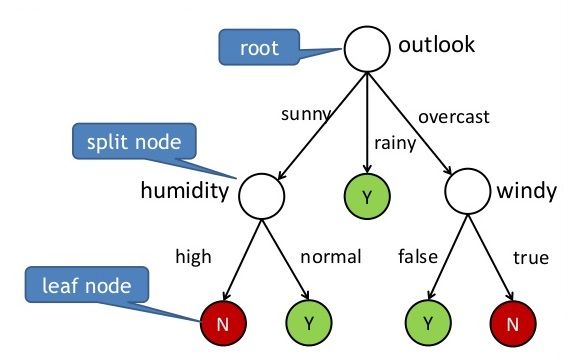
7

2.1.1   Supervised learning

A learning algorithm using supervised learning receives a set of inputs along with the corresponding
correct output to find errors. The analyst will choose one or several models, which generally has a
number of training parameters. Based on the inputs, the training algorithm op�mizes the model pa-
rameters and may update these as more data becomes available [12].
Supervised learning involves the use of labelled data. The dataset is split into three subsets: training,
test and valida�on datasets, usually in propor�on 60/20/20. A training set is used to build the model;
it contains data with labelled target and predictor variables. Target variable is a variable whose values
are to be modeled and predicted by other variables; predictor variables are the ones whose values
will be used to predict the value of the target variable [13]. A test set is used to evaluate how well the
model does with data outside the training set. The test set contains the labelled results data but they
are not used when the test set data is run through the model un�l the end, when the labelled data
are compared against the model results. The model is adjusted to minimize error on the test set.
Then, a valida�on set is used to evaluate the adjusted model on the test phase where, again, the vali-
da�on set data is run against the adjusted model and results compared to the unused labelled data.

  Figure 2. Supervised machine learning. Source [14]

If the model performs accurately using the training data but underperforms on new data, it is overfit-
�ng, i.e. the model describes the noise in the training set rather than the general patern and has too
high variance. If it performs poorly on both training and test data, it has too high bias (the model is
8

underfi�ng). Both overfi�ng and underfi�ng leads to poor predic�on on new data sets. See Figure 3
for examples of underfi�ng and overfi�ng models.

    Figure 3. Left: Model performs poorly (underfitting). Center: Model generalizes well. Right: Model is too complex and
    overfitting. Source [15]

This bias-variance trade-off is central to model op�miza�on in machine learning (Figure 4). The more
parameters are added to a model, the higher the complexity of the model, the higher variance and
the lower bias; the total error of the model raises. If the model has too few parameters (too simple
model), variance decreases while bias increases, which also leads to a high total error of the model.

    Figure 4. Bias and variance contributing to total error. Source [16]

Various techniques based on informa�on theory are used to balance variance and bias.
Supervised learning is o�en used on classifica�on and regression problems [17]. The purpose of Clas-
sification is to determine a label or category [18]. An example in healthcare is classifica�on of dermo-
scopic images into malignant and benign categories. Features, such as color, border, and homogene-
ity of the mole are extracted from the images and used for training the ML model. Eventually the al-
gorithm can provide decision support for classifying new images unseen by the algorithm.
9 Figure 5. Examples of classification problems. Source [19] Regression helps to understand how the value of the dependent variable is influenced by the changes of a selected independent variable, while keeping other independent variables constant [17]. This Figure 6. Regression model example. Source [21] method is used, for example, for predic�on of mental health costs [20]. There are many algorithms used for supervised learning. Logis�c Regression, Decision Trees, K-Near- est Neighbors, Support Vector Machines are among them. Logis�c Regression [17] Logis�c regression is best suited for binary classifica�on, i.e. datasets where output is equal to 0 or 1, and 1 denotes the default class. The method is named a�er the transforma�on func�on used in it, called the logis�c func�on h(x) = 1/(1 + e-x). In logis�c regression, the output is in the form of probabili�es of the default class. As it is a probabil- ity, the output (y-value) lies in the range of 0-1. The output is generated by log transforming the x- value, using the logis�c func�on. A threshold is then applied to force this probability into a binary classifica�on (i.e. if a value is less than 0.5, then output is 1).
10

     Figure 7. Logistic regression example. Source [22]

Decision Trees [23, 24]

A decision tree is a graph that uses branching method to show each possible outcome of a decision.
To train a decision tree, the training data is used to find which atribute best “splits” the training set
with regards to the target. A�er this first split, there are two subsets that are the best at predic�ng if
there is only the first atribute available. Then it is iterated on the second-best atribute for each sub-
set to re-split each subset. This spli�ng process con�nues un�l it has been used enough atributes to
sa�sfy the research needs.

     Figure 8. An example of decision tree. Source [25]

K-Nearest Neighbors [17, 24]

The k-nearest neighbors (kNN) method can be used for both regression and classification problems,
and uses the closest neighbors of a data point for prediction. For classification problem, the algorithm
stores all available cases and classifies new cases by a majority vote of its k nearest neighbors. The
11 case being assigned to the class is most common amongst its k nearest neighbors measured by a dis- tance function. These distance functions can be Euclidean, Manhattan, Minkowski (continuous func- tion) and Hamming distance (categorical variables). If k is equal to one, then the case is simply assigned to the class of its nearest neighbor. For regression problem, the only difference from the discussed algorithm will be using averages of nearest neighbors rather than voting from nearest neighbors. Figure 9. Example of k-NN classification. Source [26] Support Vector Machines [24, 27] Support Vector Machines (SVM) are binary classifica�on algorithms. Given a set of points of two clas- ses in N-dimensional place (where N is a number of features the data set has); SVM generates a (N-1) dimensional hyperplane that differen�ates those points into two classes. For example, there are some points of two linearly separable classes in 2-dimen�onal space. SVM will find a straight line that differen�ates points of these two classes; this line is situated between these classes and as far as pos- sible from each one. SVMs are able to classify both linear and nonlinear data. The idea with SVMs is that, with a high enough number of dimensions, a hyperplane separa�ng two classes can always be found, thereby de- linea�ng data set member classes. When repeated a sufficient number of �mes, enough hyperplanes can be generated to separate all classes in N-dimension space.
12

     Figure 10. An example of SVM work. Source [28]

Ensemble Methods [17, 24]

Ensemble means combining the predic�ons of mul�ple different weak machine learning models to
predict on a new sample. Ensemble learning algorithms have the following advantages:
           •   they average out biases
           •   they reduce the variance (the aggregate opinion of several models is less noisy than the
               single opinion of one of the models)
           •   they are unlikely to over-fit (if individual models do not over-fit, then a combination of the
               predictions from each model in a simple way (average, weighted average, logistic regres-
               sion) will not overfit)
Random Forest and Gradient Boos�ng are examples of ensemble methods.
Random Forest [23]
A random forest is the average of many decision trees, each of which is trained with a random sample
of the data. Each single tree in the forest is weaker than a full decision tree, but by pu�ng them all
together, the overall performance is beter due to diversity.

     Figure 11. An example of how Random Forest algorithm works. Source [29]
13 Gradient Boosting [23] Gradient boos�ng, like random forest, is also made from “weak” decision trees. The core difference is that in gradient boos�ng, the trees are trained one a�er another. Each subsequent tree is trained pri- marily with data that had been wrongly iden�fied by previous trees. This allows gradient boost to fo- cus on difficult cases. Figure 12. An example of gradient boosted decision tree. Source [30] 2.1.2 Unsupervised learning Unlike supervised learning, unsupervised learning is used with data sets where data is not labeled be- forehand. An unsupervised learning algorithm explores raw data to find underlying structures [12]. Figure 13. Unsupervised machine learning. Source [14] The main types of unsupervised learning problems are associa�on, clustering, and dimensionality re- duc�on [17]. Association is applied to discover the probability of the co-occurrence of items in a collec�on. For ex- ample, if an associa�on exists and how strong this associa�on is [17].
14

Clustering groups samples such that objects within the same group (cluster) are more similar to each
other than to objects in other groups (clusters) [17]. Segmentation is related to clustering. An image
is divided into several sub I regions/segments that are conceptually meaningful or simple for further
analysis in a process. Usually the goal is to locate objects and boundaries in the images. There are
various methods to do this, like clustering using K-means, compressing image to reduce texture, edge
detec�on or Markov fields. Segmenta�on process is widely used in medicine for analysis of MRI, CT,
X-ray, ultrasound images.

 Figure 14. CT image segmentation (on the left - original CT image, in the center - CT image using threshold technique,
 on the right - edge-based Segmentation of CT image). Source [31]

Dimensionality reduction means reducing the number of variables of a dataset while ensuring that
important informa�on is preserved [17].
K-means, Principal Component Analysis, and Topological Data Analysis are examples of unsupervised
learning algorithms.
K-means [17]

K-means is an itera�ve algorithm that groups similar data into clusters. It calculates the centroids of k
clusters and assigns a data point to that cluster having least distance between its centroid and the
data point. There are four steps in the k-means algorithm. Step 1 includes a choice of k value, random
assignment of each data point to any of the k clusters, and computa�on of cluster centroid for each
of the clusters. In step 2, each point is reassigned to the closest cluster centroid. In step 3, the cen-
troids for the new clusters are calculated. Then, steps 2 and 3 are repeated un�l nothing changes.
15

  Figure 15. An example of k-means clustering. Source [32]

Principal Component Analysis [17]

Principal Component Analysis (PCA) is used to make data easy to explore and visualize by reducing
the number of variables. This is done by capturing the maximum variance in the data into a new coor-
dinate system with axes called “principal components”. Each component is a linear combina�on of
the original variables and is orthogonal to one another. Orthogonality between components indicates
that the correla�on between these components is zero.
The first principal component captures the direc�on of the maximum variability in the data. The sec-
ond principal component captures the remaining variance in the data but has variables uncorrelated
with the first component. Similarly, all successive principal components capture the remaining vari-
ance while being uncorrelated with the previous component.

  Figure 16. Three original variables (genes) are reduced to a lower number of two new variables (principal compo-
  nents). Using PCA, the 2-D plane that optimally describes the highest variance of the data is identified (left). This 2-D
  subspace is then rotated and presented as a 2-D component space (right). Source [33]
16
Topological data analysis [9]
Topological data analysis (TDA) creates topological networks from the data sets equipped with a dis-
tance func�on, and by the layout process obtains a shape describing the data set. A topological net-
work consists of a set of nodes and a set of edges. There are two proper�es completely describing
how network shapes correspond to the data.
• Each node in a network corresponds to a collection of data points, not individual data points.
The collections corresponding to different nodes may overlap.
• Two nodes whose corresponding collections of data points overlap are connected by an edge.
A typical TDA pipeline consists of the following steps [34]:
1. The input is a finite set of points with a notion of distance between them.
2. A “continuous” shape is built on top of the data in order to highlight the underlying topology
or geometry.
3. Topological or geometric information is extracted from the structures built on top of the data.
4. The extracted topological and geometric information provides new features of the data. They
can be used to better understand the data (through visualization) or they can be combined
with other kinds of features for further analysis.
Figure 17. TDA visualization of clinical and billing data from total knee replacement patients. Source [35]
2.1.3 Semi-supervised learning
Semi-supervised learning is a class of supervised tasks and techniques that makes use of unlabeled
data for training: they typically require only a small amount of labeled data together with a large
amount of unlabeled data [36]. Therefore, semi-supervised learning can be regarded as a combina-
�on of unsupervised and supervised learning.
Labeling data o�en requires a human specialist or a physical experiment (a �me and cost consuming
process) while unlabeled data may be more easily available. Thus, in health applica�ons, semi-super-
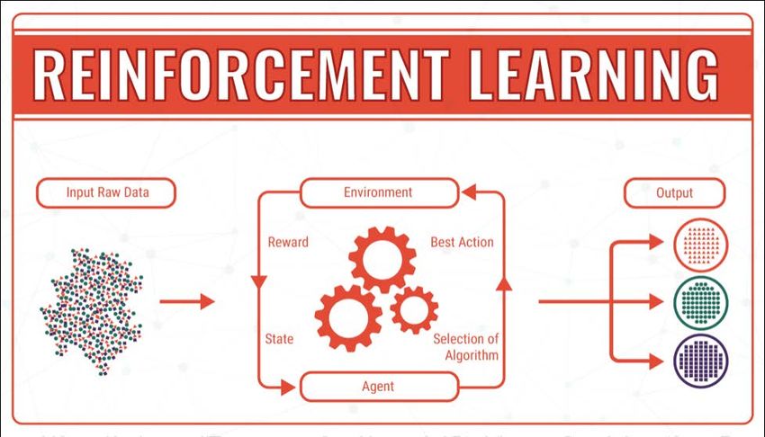
vised learning can be effec�ve due to the huge amounts of medical data required for research.17 An example of semi-supervised learning in healthcare is its use for EHR phenotype stra�fica�on. Re- searchers combined denoising autoencoders (which perform dimensionality reduc�on enabling visu- aliza�on and clustering) with random forests for classifica�on of amyotrophic lateral sclerosis sub- types and improvement of genotype-phenotype associa�on studies that leverage EHRs [37]. Read more about denoising autoencoders in sec�on Autoencoders Neural Networks. 2.1.4 Reinforcement learning Reinforcement learning is a type of machine learning algorithm that allows the machine to decide the best next ac�on based on its current state, by learning behaviors that will maximize the reward [12]. Reinforcement learning differs from standard supervised learning because correct input/output pairs are never presented. Instead, the focus is on current performance, which involves finding a balance between exploring unknown territory and exploi�ng current knowledge. In other words, reinforce- ment algorithms usually learn op�mal ac�ons through trial and error [17]. Figure 18. Reinforcement machine learning. Source [7] Supervised vs Reinforcement Learning [14] In supervised learning, a human supervisor creates a knowledge base and shares the learning with a machine. However, there are problems where the agent can perform so many different kind of sub- tasks to achieve the overall objec�ve, so that the presence of a supervisor is imprac�cal. For example in a chess game, crea�ng a knowledge base can be a complicated task since the player can play tens of thousands of moves. It is impera�ve that in such tasks the computer learns how to manage affairs by itself. It is more feasible for the machine to learn from its own experience. Once the machine has started learning from its own experience, it can then gain knowledge from these experiences to im- plement in the future moves. This is the biggest and most impera�ve difference between the con- cepts of reinforcement and supervised learning. There is a certain type of mapping between the out- put and input in both learning types. Nevertheless, in reinforcement learning there is an exemplary reward func�on that lets the system know about its progress down the right path, which supervised learning does not have.
18

Reinforcement vs. Unsupervised Learning [14]
As men�oned before, reinforcement learning has a mapping structure that guides the machine from
input to output. In unsupervised learning, the machine focuses on the underlying task of loca�ng the
paterns rather than the mapping for progressing towards the end goal. For example, if the task for
the machine is to suggest an interes�ng news update to a user, a reinforcement-learning algorithm
will look to get regular feedback from the user in ques�on, and use this feedback to build a reputable
knowledge graph of ar�cles that the person may find interes�ng. An unsupervised learning algorithm
will look at ar�cles that the person has read in the past, and suggest something that matches the
user’s preferences based on this.
Reinforcement learning is used, for example, for classifying lung nodules based on medical images
[38]. However, use of reinforcement learning in healthcare is quite challenging due to high number of
parameters that need to be tuned or ini�alized. Choosing the op�mal values for these parameters is
usually performed manually based on problem-specific characteris�cs, which is unreliable or some-
�mes even unfeasible. Moreover, it is difficult to generalize and explain both the learning process and
the final solu�on in reinforcement learning algorithms, being a “black box” problem. Read further
about algorithm/model transparency in sec�on 2.1.6 Interpretability of machine learning algorithms.

2.1.5      Neural networks

An artificial neural network (ANN) is a computational non-linear model based on the neural structure
of the brain that is able to learn to perform tasks like classification, prediction, decision-making, visu-
alization, and others just by considering examples.
An artificial neural network consists of artificial neurons (processing elements) and is organized in
three interconnected layers: input, hidden that may include more than one layer, and output (Figure
19).

     Figure 19. An example of neural network. Source [39]

If there is more than one hidden layer, the network is considered deep learning.
Deep neural networks learn by adjus�ng the strengths of their connec�ons to beter convey input sig-
nals through mul�ple layers to neurons associated with the right general concepts [40]. When data is
fed into a network, each ar�ficial neuron that fires transmits signal to certain neurons in the next
layer, which are likely to fire if mul�ple signals are received. The process filters out noise and retains
only the most relevant features.
19
There are some popular types of deep learning ANNs as
• Convolutional Neural Networks
• Deep Autoencoders
• Recurrent Neural Networks
• Deep Belief Networks
Convolu�onal Neural Networks [41]
Convolu�onal neural networks (CNN) convolves learned features with input data, and uses 2-D con-
volu�onal layers. This makes it well suited to processing 2-D data, such as images.
A CNN can have many layers where each layer learns to detect different features of an image. Filters
are applied to each training image at different resolu�ons, and the output of each convolved image is
used as the input to the next layer. The filters can start as very simple features, and increase in com-
plexity to features that uniquely define the object as the layers progress.
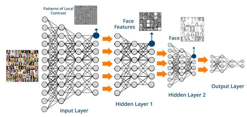
CNNs eliminate the need for manual feature extrac�on. They work by extrac�ng features directly
from data (see Figure 20). This automated feature extrac�on makes CNN deep learning models highly
accurate for computer vision tasks.
Figure 20. Example of what each layer in CNN may learn based on face image dataset. Source [42]
Autoencoders Neural Networks [43, 44]
An autoencoder is a neural network with three layers: an input layer, a hidden (encoding) layer, and
a decoding layer. The network is trained to reconstruct its inputs, which forces the hidden layer to try
to learn good representations of the inputs.
There are several types of autoencoders, but the most popular (and the basic) one is denosing autoen-
coder (DAE). To force the hidden layer to discover features that are more robust and prevent it from
simply learning the identity, the DAE is trained to reconstruct the input from a corrupted version of it.
The amount of noise to apply to the input is typically 30 percent, but in the case of very little data, the
noise percent is higher.20
Figure 21. Example of denoising autoencoder's work. Source [45]
Recurrent Neural Networks [46]
Recurring neural networks (RNN) allow for both parallel and sequential computation. An RNN is a
variant of a recursive ANN in which connections between neurons make a directed cycle. It means
that output depends not only on the present inputs but also on the previous step’s neuron state.
RNNs process an input sequence one element at a time, maintaining in their hidden units a state vec-
tor that implicitly contains information about the history of all the past elements of the sequence.
This memory allows users solve NLP problems like connected handwriting recognition or speech
recognition.
Figure 22. Example of recurrent neural network. The hidden layer forms a directed graph able to feedback infor-
mation from previous calculations. Source [45, 47]
Deep Belief Networks [44, 48, 49]
A deep belief network (DBN) is composed of mul�ple layers of latent variables (“hidden units”), with
connec�ons between the layers but not between units within each layer. When trained on a set of
examples without supervision, a DBN can learn to probabilis�cally reconstruct its inputs. The layers
then act as feature detectors. A�er this learning step, a DBN can be further trained with supervision
to perform classifica�on.
DBNs can be viewed as a composi�on of simple, unsupervised networks such as restricted Boltzmann
machines or autoencoders, where each sub-network's hidden layer serves as the visible layer for the21
next. Boltzmann Machine is an RNN with stochas�c binary units and undirected edges between units.
An RBM is a Boltzmann Machine that consists of hidden layers with connec�ons between the layers
but not between units within each layer.
Figure 23. Example of a basic deep belief network for binary classification with k hidden layers. Source [50]
Neural networks are great at solving problems where the data is highly structured. However, deep
learning applica�ons are not able to explain how they came up with their predic�ons. This “black
box” problem is quite challenging in healthcare. Doctors do not want to make medical decisions that
poten�ally might harm the pa�ent’s health and life without understanding the machine’s train of
thought towards its recommenda�ons.
2.1.6 Interpretability of machine learning algorithms
According to Miller [51], interpretability is the degree to which a human can understand the cause of
a decision. The higher the interpretability of a model, the easier it is for someone to comprehend
why certain decisions/predic�ons were made.
Molnar describes the following levels of interpretability [52]:
• Algorithm transparency (How does the algorithm create the model?)
Algorithm transparency is about how the algorithm learns a model from the data and what kind of
rela�onships it is capable of picking up. This is an understanding of how the algorithm works, but not
of the specific model that is learned in the end and not about how single predic�ons are made.
• Global, holistic model interpretability (How does the trained model make predictions?)
A model is called interpretable if one can comprehend the whole model at once [53]. To explain the
global model output, we need the trained model, knowledge about the algorithm and the data. This
level of interpretability is about understanding how the model makes the decisions, based on a holis-
�c view of its features and each of the learned components like weights, parameters, and structures.
However, it is very hard to achieve in prac�ce.
• Global model interpretability on a modular level (How do parts of the model influence pre-
dictions?)
While global model interpretability is usually out of reach, there is a beter chance to understand at
least some models on a modular level. In the case of linear models, the interpretable parts are the22
weights and the distribu�on of the features. The weights only make sense in the context of the other
features used in the model. Nevertheless, arguably the weights in a linear model s�ll have beter in-
terpretability than the weights of a deep neural network.
• Local interpretability for a group of prediction (Why did the model make specific decisions
for a group of instances?)
The model predic�ons for mul�ple instances can be explained by either using methods for global
model interpretability (on a modular level) or single instance explana�ons. The global methods can
be applied by taking the group of instances, pretending it is the complete dataset, and using the
global methods on this subset. The single explana�on methods can be used on each instance and
listed or aggregated a�erwards for the whole group.
• Local interpretability for a single prediction (Why did the model make a specific decision for
an instance?)
We can also look at a single instance and examine what kind of predic�on the model makes for this
input, and why it made this decision. Local explana�ons can be more accurate compared to global
explana�ons since locally they might depend only linearly or monotonic on some features rather than
having a complex dependence on the features.
Examples of interpretable ML algorithms are linear regression, logis�c regression, decision tree, KNN,
naive Bayes classifier, and some others.
There are several features that characterize healthcare data [54].
• Much of the data is in multiple places and in different formats
• The data can be structured or unstructured
• Definitions are inconsistent/variable: evidence-based practice and new research is developing
continuously
• The data is complex
• Regulatory requirements for data reuse are strict
Machine learning algorithms allow examining paterns in heterogeneous and con�nuously growing
healthcare data which human specialists are not capable to process in any reasonable �meframe.
Factors like growing volumes and variety of available data, computa�onal processing that is cheaper
and more powerful, affordable data storage, as well as improvements of theory and computa�onal
methods make it possible to quickly and automa�cally produce models that can analyze bigger, more
complex data and deliver faster, more accurate results.
Important benefits from machine learning within healthcare include [9]
• reduction of administrative costs
• clinical decision support
• cutting down on fraud and abuse
• better care coordination
• improved patient wellbeing/health
For more examples of successful machine learning application in healthcare, read Use cases.
However, we should also mention the challenges still to be addressed while using machine learning
technologies in healthcare [55]. The challenges are as follows:23
• Data governance. Medical data is personal and not easy to access. Many patients are not
willing to share their data due to data privacy concerns. Used improperly, such data collec-
tions, both on an individual and population levels, pose a potential threat to privacy and au-
tonomy. For more details on regulations on health data use in development of ML algorithms,
please refer to section 2.3.2 Privacy concerns in machine learning.
• Algorithm interpretability. Algorithms are required to meet the strict regulations on patient
treatment and drug development. Doctors (and patients) need to be able to understand the
causal reasoning behind machine conclusions. In general, most ML methods are «black
boxes» that offer little or no interpretability on how the results are produced. This might be a
major problem in healthcare settings. We discussed this issue more detailed in section 2.1.6
Interpretability of machine learning algorithms.
• Breaking down “data silos” and encouraging a “data-centric view”. Seeing the value of
sharing and integrating data is very important in medical research for improvement of pa-
tient treatment in the long term.
• Standardizing/ streamlining electronic health records. At present, EHRs are still messy and
fragmented across systems. Structured and standardized EHRs will provide a foundation for
better healthcare in general, and for personalized medicine in particular.
• Overdiagnosis. Healthcare is supposed to reduce illness and preventable death and improve
quality of life. Active health intervention is not always good. Sometimes health services take
people who do not need intervention, subject them to tests, label them as sick or at risk, pro-
vide unnecessary treatments, tell them to live differently, or insist on monitoring them regu-
larly. These overdiagnosis interventions produce complications, reduce quality of life, or even
cause premature death [56]. For ML, there is a concern that the development, particularly of
patient tools may lead to overdiagnosis and worries among the population – meaning in-
creased pressure on the healthcare system rather than the decrease that is often aimed for.
Machine learning and artificial intelligence are hot topics today in literally all areas where huge
amounts of heterogeneous data are available. The underlying idea is that sophisticated methodology
is needed to transform all available information into useful actions or predictions. Providing a thor-
ough description of the knowledge in the field is challenging. Bughin et al. examine how AI is being
deployed by companies that have started to use these technologies across sectors and further ex-
plored the potential of AI to become a major business disruptor [57].
2.3.1 Reasons for ML rise
The main reasons for machine learning to become a hot topic in many areas today are:
• Vast amounts of data
AI/Machine learning needs to a big amount of data in order to learn and develop itself. Nowadays,
huge data sets are available for training of ML algorithms. 2.7 zetabytes of data exist in the digital
universe today [58] (one zetabyte is equivalent to 44 trillion gigabytes). For comparison, in 1992–
2002, about 2–5 exabytes were generated per year [59] while in 2016, 2.5 exabytes were generated
per day [60].
• Increase of computational power (GPUs)24
GPU computing is the use of a GPU (graphics processing unit) as a co-processor to accelerate CPUs
for computationally and data-intensive tasks [61]. A CPU has a few cores optimized for sequential se-
rial processing while GPU consists of hundreds of smaller cores, which together allow it to perform
multiple calculations at the same time. This massively parallel architecture gives GPU its high compu-
tational performance. In the 1999-2000, computer scientists, along with researchers in fields such as
medical imaging and electromagnetics, started using GPUs to accelerate a range of scientific applica-
tions [61]; from the mid-2010s, GPU computing also powers machine learning and artificial intelli-
gence software [62].
• Improvements of theory and methods
In the book [63], Goodfellow et al. talk about the recent research in the ML field and the new meth-
ods that have been developed and refined in last decades. We explain just some of the improve-
ments mentioned by Goodfellow [63].
Greedy layer-wise unsupervised pre-training is an example of how a representation learned for one
task can be used for another task. It relies on a single-layer representation learning algorithm that
learns latent (i.e. not directly observed) representations. Each layer is pre-trained using unsupervised
learning: it takes the output of the previous layer and produces as output a new representation of
the data, whose distribution is hopefully simpler. Unsupervised pre-training can also be used as ini-
tialization for other unsupervised learning algorithms, such as deep autoencoders [64], deep belief
networks [65] and deep Boltzmann machines [66].
Transfer learning refers to the situation where what has been learned in one setting is exploited to
improve generalization in another setting. Two extreme forms of transfer learning are one-shot
learning and zero-shot learning. For one-shot learning, only one labeled example of the transfer task
is given; no labeled examples are given at all for the zero-shot learning task. In one-shot learning
[67], the representation learns first to cleanly separate the underlying classes. Next, during transfer
learning, only one labeled example is needed to infer the label of many possible test examples that
all cluster around the same point in representation space. In zero-shot learning [68-70], additional
information is exploited during training. Three random variables are available for the algorithm: the
traditional inputs, the traditional outputs, and an additional random variable describing the task.
In image analysis, if a group of pixels follows a highly recognizable pattern, even if that pattern does
not involve extreme brightness or darkness, that pattern could be considered extremely salient. To
implement such a definition of salience is to use generative adversarial networks [71]. In this ap-
proach, a generative model is trained to fool a feedforward classifier. The feedforward classifier at-
tempts to recognize all samples from the generative model as being fake and all samples from the
training set as being real. Any structured pattern that the feedforward network can recognize is
highly salient.
Among other improvements, it is a synergy of minimizing prediction error with Common Task Frame-
work (CTF). Predictive method is able to make good predictions of response outputs for future input
variables. According to Donoho [72], CTF is the crucial methodology driving the success of predictive
modeling. It consists of the following components:
• A publicly available training data set with a list of feature measurements and a class label
for each observation
• A set of enrolled competitors whose common task is to infer a class prediction rule from the
training data
• A scoring referee, to which competitors can submit their prediction rule. The referee runs the
prediction rule against a testing dataset and objectively and automatically reports the predic-
tion accuracy achieved by the submitted ruleYou can also read