Hierarchical control and learning of a foraging CyberOctopus
←
→
Page content transcription
If your browser does not render page correctly, please read the page content below
Hierarchical control and learning of a foraging CyberOctopus
                                         Chia-Hsien Shih, Noel Naughton, Udit Halder, Heng-Sheng Chang,
                                         Seung Hyun Kim, Rhanor Gillette, Prashant G. Mehta, Mattia Gazzola*

                                         Chia-Hsien Shih, Heng-Sheng Chang, Seung Hyun Kim, Prashant G. Mehta, and Mattia Gazzola
                                         Department of Mechanical Science and Engineering
                                         University of Illinois at Urbana-Champaign
                                         Urbana, IL 61801
                                         Email Address: mgazzola@illinois.edu
                                         Noel Naughton
                                         Beckman Institute for Advanced Science and Technology
                                         University of Illinois at Urbana-Champaign
arXiv:2302.05811v1 [cs.RO] 11 Feb 2023

                                         Urbana, IL 61801
                                         Udit Halder
                                         Coordinated Science Laboratory
                                         University of Illinois at Urbana-Champaign
                                         Urbana, IL 61801
                                         Rhanor Gillette
                                         Department of Molecular and Integrative Physiology
                                         University of Illinois at Urbana-Champaign
                                         Urbana, IL 61801

                                         Keywords: Bioinspiration, Soft robotics, Hierarchical control

                                        Abstract. Inspired by the unique neurophysiology of the octopus, we propose a hierarchical framework that simplifies the
                                    coordination of multiple soft arms by decomposing control into high-level decision making, low-level motor activation, and local reflexive
                                    behaviors via sensory feedback. When evaluated in the illustrative problem of a model octopus foraging for food, this hierarchical
                                    decomposition results in significant improvements relative to end-to-end methods. Performance is achieved through a mixed-modes
                                    approach, whereby qualitatively different tasks are addressed via complementary control schemes. Here, model-free reinforcement
                                    learning is employed for high-level decision-making, while model-based energy shaping takes care of arm-level motor execution. To render
                                    the pairing computationally tenable, a novel neural-network energy shaping (NN-ES) controller is developed, achieving accurate motions
                                    with time-to-solutions 200 times faster than previous attempts. Our hierarchical framework is then successfully deployed in increasingly
                                    challenging foraging scenarios, including an arena littered with obstacles in 3D space, demonstrating the viability of our approach.

                                     1     Introduction
                                     Soft materials have long been seen as key drivers for improving robots’ abilities to interact with and adapt to
                                     their environments [1, 2, 3]. Nonetheless, it is precisely the advantages afforded by physical compliance that, in
                                     turn, render soft robots difficult to control. Indeed, material non-linearities, instabilities, continuum mechanics,
                                     distributed actuation, and conformability to the environment all render the control problem challenging [4, 5]. In
                                     search of potential solutions, roboticists have turned to nature for inspiration [6], from the investigation of elephant
                                     trunks [7, 8], mammalian tongues [9, 10], and inchworms [11, 12, 13] to plant tendrils [14, 15], starfish [16, 17],
                                     snakes [18, 19], and octopuses [20, 21, 22, 23, 24, 25, 26]. The latter, in particular, have received a great deal of
                                     attention owing to their unmatched ability to orchestrate multiple soft arms for swimming, crawling, and hunting,
                                     as well as manipulating complex objects, from coconut shells to lidded jars [27, 28].
                                        Within this context, a potential solution framework based on hierarchical decomposition is suggested by the
                                    unique neurophysiology of the octopus. In contrast to the mostly centralized brain structure of vertebrates [29],
                                    the octopus exhibits a highly distributed neural system wherein two thirds of its brain lies within its arms [30].
                                    This Peripheral Nervous System (PNS) is organized into brachial ganglia, colocated with the suckers, and is
                                    responsible for low-level sensorimotor tasks and whole-arm motion coordination [31]. Indeed, surgically severed
                                    arms are known for being able to execute motor programs such as reaching or recoiling [32, 33]. The Central
                                    Nervous System (CNS), composed of the remaining third of the neural tissue, is instead located in the mantle and
                                    is thought to be responsible for learning and decision making by integrating signals from the entire body [34]. This

                                                                                                        1
(a) Central brain                  Behavioral primitives         (b) Foraging Problem

                             Central
                              level
                                                                     Central-level coordination          Food
                                                                          Reach / Crawl                       Obstacle
                                          Motor primitives

                             Arm
                             level
                                                                                                             Local
                                        Outsource to physics                                              environment
 Peripheral brain
                             Local
                                                                       Arm-level coordination
                              env.                                                                         modulation
    in the arms                                                       Distributed muscle control

Figure 1: (a) Our proposed control hierarchy inspired by the distributed neurophysiology of the octopus: a centralized decision-maker selects appro-
priate motion primitives, arm-level controllers generate the necessary muscle activations and physical compliance accommodates for environmental
obstacles. (b) A CyberOctopus foraging for food in the presence of obstacles.

neural architecture is naturally suggestive of a control hierarchy wherein high-level decisions are made in the CNS,
executed by the PNS, and finally modulated by the local environment via arm compliance.
   Reflecting these considerations, we present a tri-level hierarchical approach to coordination and learning in an
octopus computational analog, henceforth referred to as the CyberOctopus. Our framework, illustrated in Fig. 1,
decomposes control into central-level, arm-level, and local environment-level. At the central level, executive and
coordination decisions (behavioral primitives), such as reaching for food or crawling, are taken and issued to the
individual arms. This top level is implemented as a compact, feedforward neural network. At the level of the
arm, modeled as an elastic slender filament, muscle activations (motor primitives) realize incoming commands
and produce appropriate deformations [25]. Muscle control is obtained via a fast energy shaping technique that
minimizes energy expenditure [35]. We supplement this control with distributed, local behavioral rules that conspire
with the arm’s compliant physics to autonomously accommodate for solid environmental features.
    The CyberOctopus is shown to learn to forage for food in increasingly challenging scenarios, including an arena
littered with obstacles in 3D space. Overall, this work illustrates how hierarchical control is not only viable in soft
multi-arms systems but, in fact, can significantly outperform end-to-end, deep-learning approaches.

2     The CyberOctopus model
Of all the elements that comprise a real octopus, here we focus on its arms and their coordination. The arms of the
CyberOctopus (Fig. 2) are modeled as linearly tapered Cosserat rods, which are slender, one-dimensional elastic
structures that can undergo all modes of deformation — stretch, bend, twist, and shear — at every cross section
[36]. Each arm is then represented as an individual passive rod upon which virtual muscles produce forces and
couples. We consider each arm deforming in-plane on account of two longitudinal muscle groups (LM1 and LM2)
and one set of transverse muscles (TM), reflecting the octopus’ physiology, as illustrated in Fig. 2a,b. Longitudinal
muscles (Fig. 2c) are located off-center from the arm’s axis of symmetry but run parallel to it, generating both forces
and couples that can cause the arm to contract (symmetric co-contractions) or bend (asymmetric co-contractions).
Transverse muscles (Fig. 2d) are located along the arm’s axis but are oriented orthogonally, so that their contraction
causes the arm to extend due to incompressibility. Oblique muscles, whose main function is to provide twist [37],
are not considered here as they are not relevant for planar motion.
   Kinematics. In the Cosserat rod formalism (Fig. 2b), each arm is described by its midline position vector
x(s, t) ∈ R2 within the plane spanned by the fixed orthonormal basis {e1 , e2 } and along the arclength s ∈ [0, L0 ],
where L0 is the arm’s rest length, and t is time. The arm’s local orientation is described by the angle θ(s, t) ∈ R
which defines the local orthonormal basis {a, b} with a = cos θ e1 + sin θ e2 and b = − sin θ e1 + cos θ e2 . The local
deformations of the arm — stretch (ν1 ), shear (ν2 ), and bending (κ) — are defined by the kinematics of the arm
                                                      ∂s x = ν1 a + ν2 b,         ∂s θ = κ                                                     (1)

For a straight arm at rest, ν1 = 1 and ν2 = κ = 0.

                                                                         2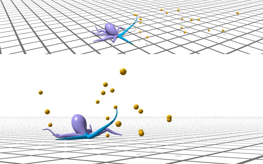
(a) (b) LM1
Virtual muscles
1
TM LM2
TM
LM
2 Cosserat rod model
(c) LM1 activation (d) TM activation
Arm shortens or bends
Arm elongates
Arm rests Arm rests
Longitudinal muscle (LM)
Transverse muscle (TM)
Figure 2: (a) Histological cross-section of an Octopus rubescens arm showing the longitudinal (LM1 and LM2) and transverse (TM) muscles.
Muscles are labeled in red by phalloidin staining (Image credit: Tigran Norekian and Ekaterina D. Gribkova). (b) Accordingly, our model arm
consists of top (LM1, blue) and bottom (LM2, orange) virtual longitudinal muscles as well as virtual transverse muscles (TM, green). The soft
arm itself is represented as a single Cosserat rod, to capture its passive elastic mechanics. Muscle activations are defined along the arm. (c)
Longitudinal muscle activations result in arm shortening (symmetric co-contraction) or bending (asymmetric co-contraction), while (d) transverse
muscle activations result in arm elongations, due to tissue incompressibility.
Dynamics. The dynamics of the planar arm [38, 25] read
ρAv1 cos θ − sin θ n1 v1
∂
∂t ρAv2 = s sin θ cos θ n2 − ζ v2 (2)
ρIω ∂s m + ν1 n2 − ν2 n1 ω
where v = (v1 , v2 ) and ω are the linear and angular velocity of the arm, respectively, ρ is the density of the arm,
A and I are the arm’s local cross-sectional area and second moment of area, n = (n1 , n2 ) and m are the internal
forces (in the local frame) and couples along the arm, and ζ > 0 is a damping coefficient capturing viscoelastic
effects. The arm dynamics (Eq. 2) are accompanied by a set of fixed/free type boundary conditions for all t ≥ 0
(fixed) x(0, t) = x0 , θ(0, t) = θ0
(3)
(free) n(L0 , t) = 0, m(L0 , t) = 0
where x0 ∈ R2 and θ0 ∈ R are the prescribed position and orientation of the arm at its base. Since the arm is
freely moving, a free boundary condition at the tip is chosen.
Internal stresses. The overall internal forces and couples acting on the arm (n, m) encompass both passive
and active effects
X X
n = ne + nm , m = me + mm (4)
m∈M m∈M
where (ne , me ) are restoring loads due to passive elasticity, and (nm , mm ) are the active loads resulting from the
contraction of muscle m ∈ M , with M = {LM1, LM2, TM} being the collection of muscle groups in the arm.
For a linearly elastic arm, passive elastic forces and couples read
e EA(ν1 − 1)
n = , me = EIκ (5)
GAν2
where E and G are Young’s and shear moduli.
The contraction of a muscle m ∈ {LM1, LM2, TM} is modeled via the activation function αm (s, t) ∈ [0, 1], with
1 corresponding to maximum activation (Fig. 2c,d). When virtual muscles contract, they produce on the arm a
distributed force nm (s, t) (in the local frame) that depends on the musculature’s spatial organization. We model
this as
m m m m
m α σ A T
n = (6)
0
3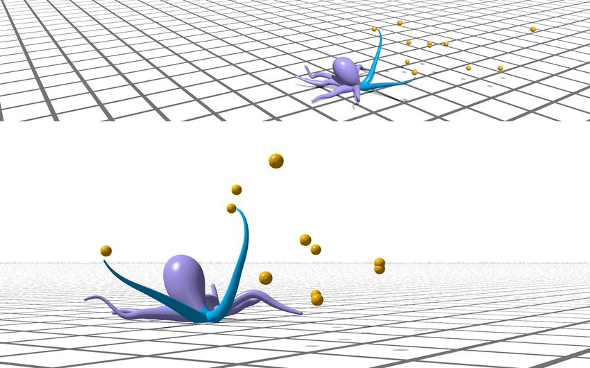
where σ m is the maximum stress generated by the muscle, Am is its cross sectional area, and Tm accounts for the
musculature configuration. For longitudinal muscles, TLM = 1 since contractions directly translate into compression
forces along the arm (note that due to small shear ν2 ≈ 0 — confirmed numerically — the vector a of Fig. 2b
effectively coincides with ∂s x). For transverse muscles, TTM = −1, capturing the fact that their contractions cause
radial shortening, which in turn extends the arm due to incompressibility (Fig. 2d). Additionally, the muscles’
force-length relationships are modeled here as a constant function, however, more complex descriptions can be
incorporated [25].
   Due to the offset location of the longitudinal muscles with respect to the arm’s main axis, the active forces
nLM generate couples (mLM ), which are modeled as follows. We denote the position of a muscle relative to the
arm centerline by the vector xm (s) = ±φm (s)b, where φm (s) is the off-center distance (Fig. 2b). The positive and
negative signs are associated with LM1 and LM2, respectively. Then the resulting couples are
                                 mm = (xm × nm ) · (e1 × e2 ) = ±φm αm σ m Am Tm                                    (7)
Transverse muscles are arranged perpendicularly to the arm (Fig. 2d), and thus result in no couples (mTM = 0).
   Static configurations. For a static muscle activation αm (s), the equilibrium configuration of the arm is
characterized by the balance of forces and couples. This is obtained by equating the right-hand side of the
dynamics (2) to zero, yielding
                                             e         X  nm
                                              n
                                                    = −
                                             me                mm
                                            | {z }      m∈M                                              (8)
                                                        |
                                              Elastic arm
                                                             {z   }
                                            passive response         Muscle
                                                                   contractions
Equation 8 is solved for the static strains ν1 , ν2 , κ, which in turn lead to the equilibrium configuration of the arm,
obtained by integrating the kinematics of Eq. 1.
   While Eq. 8 suffices to determine the equilibrium configuration for given muscle activations αm (s), it does
not account for the dynamical response of the arm transitioning between activations, all the while experiencing
environmental loads. To remedy this, we evaluate the effect of muscle activations (and thus of the control policies
that determine them) in Elastica [36, 39, 40], an open-source software for simulating the dynamics of Cosserat rods
(Eq. 2). Elastica has been demonstrated across a range of biophysical applications from soft [40] and biohybrid
[39, 41, 42, 43] robots to artificial muscles [44] and biolocomotion [39, 18, 35, 25]. In Elastica, our CyberOctopus
consists of a head and eight arms, of which only a subset (gradually increased throughout the paper) is actively
engaged. Material and geometric properties of our model octopus are determined from typical literature values [45]
as well as experimental characterizations of Octopus rubescens [35]. Numerical values and details of our muscle
models are provided in SI Tables 1-3 and in [25].

3     Arm-level problem: motor execution
Octopuses perform certain goal-directed arm motions via templates of muscle activations, such as traveling waves of
muscle contractions [32]. These templates are encoded into the arm’s peripheral nervous system as low-level motor
programs that are selected, modulated, and combined together to achieve basic behaviors such as reaching and
fetching [46, 32, 47]. Inspired by this, we define two types of primitives for inclusion in our hierarchical approach:
motor primitives (Sec. 3.1) and behavioral primitives (Sec. 4.1). Motor primitives are low-level motor programs
that coordinate the contraction of the CyberOctopus’ muscles to accomplish a stereotypical motion. Behavioral
primitives are sequences of motor primitives whose combination enables the completion of simple goal-directed
tasks (here crawling or reaching available food). These behavioral primitives can then be further composed into
more complex behaviors, such as foraging.

3.1   Motor primitives: Reaching to a point in space
We focus on a motor primitive that efficiently moves the tip of the arm to a specified location q ∈ R2 . This basic
motion can be used to accomplish a variety of tasks, for example reaching to a food target, fetching food to the
mouth, or crawling.
   Energy shaping (ES). To effect this motor primitive, we employ the energy shaping methodology [48, 49, 50].
As developed in our prior work [35, 25, 51], an energy shaping control law is derived to determine the static
                                                               4
muscle activations α = {αm }m∈M that cause the tip of the arm to reach a target location. The equilibrium arm
configuration that achieves this goal is obtained by solving an optimization problem that minimizes the tip-to-target
distance δ(α, q) = |q − x(L0 )| along with the muscle activation cost [25]
muscle cost task specific cost
z }| { z }| {
Energy Z L0
Shaping minimize J(α; α0 , q) = |α(s) − α0 (s)|2 ds + µtip δ(α, q) (9)
α(·); αm (s)∈[0,1] 0
(ES)
where α0 are the initial muscle activations, and µtip is a constant (regularization) coefficient. The tip-to-target
distance δ(α, q) is computed using the kinematic constraints of Eq. 1 and equilibrium constraints of Eq. 8.
Fast neural-network energy shaping (NN-ES). While we previously demonstrated the use of energy
shaping (ES) for muscle coordination in a soft arm [35, 25, 51], the solution to the above optimization problem is
reliant on a computationally expensive forward-backward iterative scheme. Here, in a hierarchical context where
energy shaping will be frequently called upon by a high-level controller, fast solutions are instead imperative.
In response to this need, we replace the forward-backward scheme with a neural network and directly learn the
mapping π : {q, α0 (s)} 7→ α(s) that takes initial muscle activations α0 (s) and target location q, and outputs the
activations α(s) that cause the arm to reach q while minimizing muscle costs (Fig. 3a).
In the CyberOctopus’ arm, muscle activations are continuous over s ∈ [0, L0 ], requiring us to first obtain a finite-
dimensional representation of the activations for use with our neural network, which we accomplish via a set of K
orthonormal basis functions {ek (s)}Kk=1 . The procedure for finding this set is described in the SI. In this P basis set,
the continuous muscle actuation profile α(s) is represented by the coefficients {α̂k }K k=1 , so that α(s) = k α̂k ek (s).
The inputs to the network are then the coefficients of the initial actuation profile {α̂0,k } along with the target
location q. Denoting the network weights as v, the outputs of the network are then the coefficients of the desired
muscle activation profile {α̂k (v)}. The loss function of the network is then obtained by recouching Eq. 9 as a
function of the network weights v
Neural-Network XK XK
!
Energy Shaping minimize J α̂k (v)ek (s); α̂0,k ek (s), q (10)
v
(NN-ES) k=1 k=1
Individual muscles’ activation bounds (αm (s) ∈ [0, 1]) of Eq. (9) are enforced via the function max(min(αm (s), 0), 1).
3.2 An arm reaching for food
To enable our arm, we train the mapping π, represented as a feedforward neural network with three hidden layers of
128 Rectified Linear Unit (ReLU) activation functions. This process can be summarized as follows. The network is
trained for 4000 epochs. For each epoch, 100 training samples are generated with initial activations α0 (s) randomly
selected from a Gaussian distribution, and target locations q (food) randomly selected from a uniform distribution
over the workspace W (the set of all points reachable by the tip of the arm). For each training sample, the neural
network produces an α(s, v), from which the target-to-tip distance δ(α(s, v), q) is computed based on the resulting
equilibrium configuration (Eq. 8 and Eq. 1). Because δ directly depends on the neural network weights v — through
α(s, v) — we can compute the gradient of Eq. 10 with respect to v and thus update π in an unsupervised manner.
As seen in Fig. 3a, the network successfully learns, minimizing the loss function of Eq. 10. Exploring the
characteristics of the learned mapping, we find that the initial configuration of the arm plays a substantial role
in determining muscle activation costs (Fig. 3b). For a straight initial configuration (|α0 (s)|2 = 0), targets in
the middle of the workspace require less change in muscle activation. Indeed, the arm can reach these targets
by activating only the longitudinal muscles along the arm’s distal end, which is thinner and hence less stiff. In
contrast, targets at the boundary of W require recruiting both longitudinal and transverse muscles to bend the
base (thick and stiff) and extend the arm. For a bent initial configuration, the change in muscle energy is generally
lower since longitudinal muscles are already partially activated. This is particularly true for reaching the center of
the workspace.
We next proceed to compare our NN-ES approach with the original iterative ES [25], employing the termi-
nation conditions of normalized tip-to-target distance δ(α, q)/L0 < 0.01% or 10,000 maximum iterations. To
quantify differences in the obtained equilibrium configurations x(s), we introduce the similarity metric D =
5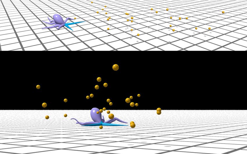
Training                      Energy cost +                                      Dynamics                             Learning curve
(a) NN-ES structure
                                                             Distance error                        Loss
                                  Target                                       Update

                                                                                                                                              Loss
                                  position                          Neural
                                                Current            Network               Predicted muscle
                                                                                                              Apply energy
                                                 muscle                                     activations
                                                                                                             shaping control
                                               activations
                                                                                                                                                             Epochs
                                          Normalized energy
                                                                                          Similarity: 0.97                 Similarity: 0.89

                                                                    (c) Configurations
                                    From rest configuration                                        Workspace

                                                                                                                                                     Similarity
(b) Muscle energy cost field

                                           High cost                                                 Target
                                                                                                    ES
                                      Workspace                                                           NN-ES
                                                   Low cost

                                                                                          Time cost (s)          Distance to target (%)         Normalized energy
                                    From bent configuration
                                                                    (d) Performance

                                      Low cost
                                                       High cost

     Figure 3: Arm-level controller: (a) Neural Network Energy Shaping (NN-ES) control utilizes a learned mapping to determine static muscle
     activations, and dynamically brings the arm to a given food target. The mapping, represented as a neural network, is trained to take as inputs the
     food target location and current muscle activations, and then outputs muscle activations that minimize tip-to-food distance and energy expenditure.
     (b) Muscle energy-cost (Eq. 9) normalized by arm length shows the cost of NN-ES to reach a point within the workspace W given the starting arm
     configuration (top panel–initially straight arm, bottom panel–initially bent arm). (c) NN-ES obtained solutions have high similarity relative to
     iterative ES solutions [25]. Differences may arise when targets are located towards the edge of the workspace. Indeed, arm configurations obtained
     via NN-ES are observed to bend near the tip, while ES solutions bend closer to the base. Right panel shows box plot of similarity score between
     NN-ES and iterative ES solutions, with orange line representing the median, purple box representing the inter-quartile (middle 50%) range, and
     whiskers denoting the min and max of 100 evaluation samples. (d) Performance of NN-ES and iterative ES, the latter considering an increasing
     number of iterations in termination condition. Orange lines represent the metric’s median value, boxes represent the inter-quartile (middle 50%)
     range, and whiskers denote the min and max of 100 evaluation samples. Comparison shows NN-ES achieves solutions over 200x faster than the
     iterative ES scheme, while achieving median tip-to-food distances (normalized by the arm length) of less than 1%. The median muscle energy cost
     of iterative ES increases with the max number of iterations allowed. This reflects the fact that obtained solutions improve with more iterations,
     decreasing the tip’s distance to the target, often through bending and thus higher actuation costs. NN-ES has slightly higher median energy cost
     (and similar maximum energy cost) as the most accuracy iterative ES solution.
           RL                          −1
        1 + 0 0 xNN-ES (s) − xES (s) ds     ∈ (0, 1], where 1 indicates identical solutions. As seen in Fig. 3c, for 100
      randomly generated cases, NN-ES and ES produce solutions characterized by a high degree of similarity (average
      D = 0.89). Differences appear for targets located far from the base, with NN-ES stretching and bending the
      arm towards the tip, while ES directly orients the entire arm in the food direction. Both algorithms are accurate
      in reaching food, achieving median tip-to-target distances of less than 1% relative to the rest length of the arm,
      although we note that NN-ES tends to utilize slightly larger muscle activations than ES (Fig. 3d). This drawback
      is nonetheless compensated by a significant reduction in solution time (Fig. 3d), whereby NN-ES outperforms ES
      by a factor of 200. Further, we note that while ES performance may depend on the allowed maximum number
      of iterations, the trends described above persist as we span from 100 to 10,000 max iterations. Taken together,
      these results demonstrate NN-ES to be fast and accurate in coordinating muscle activity and in executing low-level
      reaching motions. We thus conclude that NN-ES is suitable to be integrated into our hierarchical approach.

      4                        Central-level problem: coordinating foraging behavior
     We now turn to the problem of a CyberOctopus foraging for food within a two-dimensional (planar) arena (Fig. 1b).
     Inspired by real octopuses coordinating their arms to move and collect food [28, 52], the CyberOctopus is tasked
     with maximizing the energy intake derived from collecting food, while minimizing the muscle activations required
     to reach for it. By engaging its multiple arms, the CyberOctopus can move in any planar direction without re-
                                                                                                       6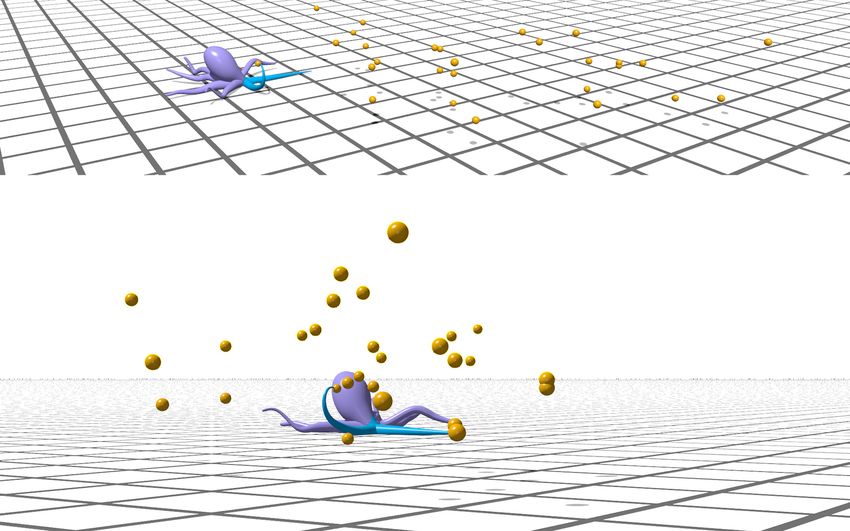
orienting its body. This multi-directionality, compounded by the difficulties associated with distributed muscular
actuations across multiple arms, muscle expenditure estimation, limited workspace, and potential presence of solid
obstacles, renders the foraging problem challenging.
   Here, we define the behavioral primitives available to the central-level controller for orchestrating foraging
behavior (Sec. 4.1), before providing the full problem’s mathematical formulation (Sec. 4.2). Finally, we describe a
reinforcement learning-based approach (Sec. 4.3) that utilizes a spatial attention strategy to simplify the planning
process, allowing us to successfully control the CyberOctopus.

4.1   Behavioral primitives: reach all and crawl
The combination of low-level motor primitives into ordered sequences allows us to construct basic behavioral
primitives. We define two behavioral primitives, reach all and crawl, in an attempt of abstracting out the complexity
of foraging into simple terms. Nonetheless, our decomposition approach conveniently provides the opportunity and
freedom of defining arbitrary command sets, and different choices may be made.
    The reach all behavior consists in the arm attempting to reach all food targets within its workspace W. Food
is collected sequentially with the ordering determined in a greedy manner. The arm calculates — via the NN-ES
controller — the change in muscle activation needed to collect each food target from its current configuration, and
then collects the target that requires the least change. This process is repeated until all food in W is collected (or
attempted to).
   The crawl behavior consists of a predefined set of muscle activations αcrawlTM . First, transverse muscles are

activated to extend the arm horizontally by a fixed amount ∆r along the crawling substrate. After extension,
suckers at the tip of the arm engage with the substrate and transverse muscles are relaxed, pulling the octopus
forward by the amount ∆r, at which point the suckers are released. We note that even though we do not explicitly
model the suckers, their effect is accounted for by appropriately choosing the arm boundary conditions.

4.2   Mathematical formulation of the foraging problem in hierarchical form
Let us consider a CyberOctopus with I active arms aiming to collect T food items that are scattered randomly
throughout an arena. Food can be found at any vertical location, while the horizontal coordinates are constrained
to a two-dimensional Cartesian grid formed by discrete crawling steps (Fig. 4a). With respect to the bases of the
arms, the location of the j-th target is denoted as qj ∈ R3 . If the CyberOctopus has complete knowledge of all T
food item’s locations, the problem for the CyberOctopus is to create an optimal plan that sequentially composes
the behavioral primitives — reach all and crawl — for all of the I arms, so as to fetch all of the food, while
minimizing muscle energy expenditure.
   Before we model the full problem mathematically, it is useful to examine the simplest case of only one active
arm where all targets are within the arm’s workspace W. In this case, the CyberOctopus can simply execute a
single reach all behavior to gather all the targets. However, in cases where some of the targets lay outside W,
the CyberOctopus will also need to crawl. Depending on the location of the targets, it may be beneficial for the
CyberOctopus to crawl even if there are already targets in its workspace. Doing so may serve to bring additional
targets within reach, to gather them all more efficiently with a single reach all maneuver.
    We formulate this optimal planning problem as a Markov Decision Process (MDP). Even though time has been
continuous so far, for the MDP model we consider a discrete-time formulation. Temporal discretization naturally
arises by considering the time elapsed between the start and the end of a primitive. Since the motor primitives
are nested inside a behavioral primitive (as described in Section 4.1 and Fig. 4b), we introduce two different
discrete-time indices, at the behavioral (n) and at the motor primitive level (n̂).
   Thus, at time n, each arm executes a behavioral primitive (action) ui [n], i = 1, ..., I, which takes value in
the set {reach all, crawl}. This means that each individual arm is treated as functionally equivalent, reflecting
the observed bilateral symmetry of octopus arms [53], and tries to either reach all available food targets in its
workspace Wi , or crawls a fixed amount di along its own direction (where |di | = ∆r). As a consequence, multiple
reaching planes become simultaneously accessible, rendering the foraging problem three-dimensional. Taking the
actions of all arms together, the decision variable at time n is denoted as u[n] = {ui [n]}Ii=1 .

                                                          7
(a)                                                                          (b)                   Hierarchical control
          Target                                                                                            Central-level
                                                              Attention                                    (Reinforcement learning)

                                                              space                                                            Behavioral
                                                                                                                               primitives
                                                                                                               Arm-level
                                                                                                            NN-ES
                                                                                                          (motor primitive)

                                                                              (c)                    End-to-end control
                                                                                                           Deep network

                                 nce Δr
                  Crawl dista

Figure 4: (a) Setup of the foraging problem showing the CyberOctopus surrounded by food targets arranged on a grid whose spacing matches the
distance traveled during one crawl step. The yellow dome shows the attention space heuristic described in Sec. 4.3, so that the CyberOctopus
only considers food items within this space. (b) Block diagram for hierarchical controller (Sec. 4.2, 4.3) and (c) end-to-end controller (whose
mathematical formulation can be found in the SI). Both approaches make use of the spatial attention heuristic, and receive the same inputs to
produce one activation output. However, the hierarchical decomposition allows us to rewire internally the flows of information, separating concerns
into qualitatively different tasks, which can then be efficiently solved by appropriate algorithms.

    The state at time n is denoted as z[n]. Its components are
                                                          z[n] = {qj [n], fj [n]}Tj=1                                                        (11)
where the flag fj [n] ∈ {0, 1} signifies whether the j-th target has already been collected (fj [n] = 0) or not (fj [n] = 1).
The dynamics then become
                                                              I
                                                              X
                                     qj [n + 1] = qj [n] −          di 1(ui [n] = crawl)
                                                              i=1
                                                                                                                                             (12)
                                                        I
                                                        Y
                                     fj [n + 1] = fj [n] (1 − 1(ui [n] = reach all & qj ∈ Wi ))
                                                           i=1

where 1(·) is the indicator function. Here the first equation expresses the change in the positions (relative to the
arm base) of food targets after a crawl step, while the second term denotes the change in collection status of food
targets after a reach all step. When executing the selected behavioral primitives, the CyberOctopus first reaches
with any arm that selected reach all, before performing any crawling. Finally, the CyberOctopus is not allowed to
crawl through the boundaries of the arena. If a boundary is approached, the CyberOctopus remains in place unless
it chooses to crawl alongside or backtracks.
    Subject to the dynamics of Eq. 12, the CyberOctopus aims to find the optimal sequence of behavioral primitives
ū := {u[0], u[1], u[2], . . . , u[N − 1]} so as to maximize the cumulative reward
                                                           N
                                                           X −1
                                          max J(ū) =             R(z[n], u[n])
                                            ū
                                                            n=0
                                                                                                                                             (13)
                                        subject to        the dynamics (Eq. 12) and given z[0]
where N is a given stopping time.
  The reward function is chosen to capture the trade-off between negative energy expenditure associated with
muscle activation, and positive energy associated with food collection. It is defined as
                                               I
                                                  (
                                              X    −E c                  if ui [n] = crawl
                     R(z[n], u[n]) = −Φ[n] +          r
                                                                                                        (14)
                                              i=1
                                                   −Ei [n] + γfWi [n] if ui [n] = reach all

                                                                         8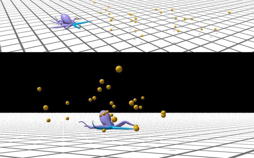
where E c and Eir [n] are the total muscle activation costs of the multiple low-level motor primitives necessary to
complete the selected command ui [n] for the i-th arm, γ is the energy of an individual food target, fWi [n] is the
total number of food items collected during a reach all execution by the i-th arm, and Φ[n] is a penalty term if all
I active arms choose reach all when no food is available.
    If ui [n] = reach all is selected, then the muscle activation sequence {αi [n̂ = 1], αi [n̂ = 2], ..., αi [n̂ = fˆWi [n]]}
is generated for reaching all food targets in the workspace Wi (as described in Section 4.1, where n̂ denotes the
discrete-time at the motor level, and fˆWi [n] is the total number of food items within reach at time n). If instead
                                                  TM is recruited. Corresponding muscle activation costs are defined
ui [n] = crawl, then the predefined activation αcrawl
as
                                                       Z L0
                                                c   1          TM
                                                                        2
                                               E =            αcrawl      ds
                                                    L0 0
                                                       Z L0 fˆW i
                                                                  [n]                                                     (15)
                                             r      1         X                 2
                                           Ei [n] =                   |∆αi [n̂]| ds
                                                    L0 0
                                                                  n̂=1

where ∆αi [n̂] = max{αi [n̂] − αi [n̂ − 1], 0} is the difference between successive muscle activations. The maximum
operator is used so that only actions leading to increased muscle activation are accounted for, i.e. there is no cost
for relaxing muscles. If the low-level controller collects all food targets within reach (which is generally true if no
obstacles are present) then fWi [n] = fˆWi [n].

4.3    Spatial attention heuristic and Reinforcement Learning solution method
In general, the high-level problem of Eq. 13 has no analytical solution. We then resort to searching for an ap-
proximate one, incorporating further insights from the octopus’ behavior. Octopuses integrate visual, tactile, and
chemo-sensory information to forage and hunt. However, in the wild they are thought to primarily rely on visual
cues [54]. For example, during foraging, they make behavioral decisions based on their distance from the den
[55], and they are able to discriminate between objects based on size, shape, brightness, and location [56]. These
observations suggest the potential use of target prioritization strategies based on spatial location.
   Adopting this insight, we define a cognitive attention heuristic wherein the CyberOctopus only pays attention
to uncollected food targets that are within the attention space V, ignoring all others. This attention space V
can be flexibly defined depending on the task at hand (see SI for details). Here, we use an attention space that
extends out twice the workspace distance (Fig. 4a). The CyberOctopus’ cognitive load can be further relieved by
considering a fixed, maximum number of closest targets, allowing for immediate planning, while retaining sufficient
environmental awareness for adequate longer-term decision-making. With this heuristic, the state of Eq. 11 reduces
to
                                                 z[n] = {qj [n]}Fj=1                                           (16)
where {qj [n]}Fj=1 are the positions (relative to the arm base) of the F closest uncollected food targets within V. If
fewer than F targets are within the attention range, the excluded entries are set to 0. If more than F targets are
within the attention range, only the first F are considered. This state definition is the one employed throughout
the remainder of the paper and is the one depicted in Fig. 4b.
   The use of this heuristic leads to a fixed state-space size, making the problem naturally amenable to reinforcement
learning approaches. Here we employ the Proximal Policy Optimization (PPO) algorithm [57], considered to be a
state-of-the-art on-policy reinforcement learning scheme due to its robust performance. PPO utilizes an actor-critic
architecture where an actor network encodes the control policy, while a critic network estimates the quality of the
control policy. Throughout the rest of the paper, the control policy is encoded in a feedforward neural network
with three hidden layers (32 × 32 × 16) of ReLU activation functions. The critic network shares the first two hidden
layers with the control policy network but has a separate third hidden layer, also with 16 neurons.

5     A CyberOctopus foraging for food
Next, we put to the test the combined machinery described in Sections 3 and 4 by simulating and characterizing a
CyberOctopus foraging for food. To illustrate the use of primitives for high-level planning and reasoning, we first
consider the reduced problem of a single active arm (Sec. 5.1), for which an analytical solution can be obtained under
                                                              9
(a) Demonstration (c) Performance
Hierarchical End2end
structure
(Eq. 13 w/o penalty)
PPO Greedy
Q
Net energy
Random
Avg. time steps per
collected food item
(b) Learning curve PPO Q Greedy Random
Avg. crawl steps per
collected food item
Return
Epochs PPO Q Greedy Random E2E
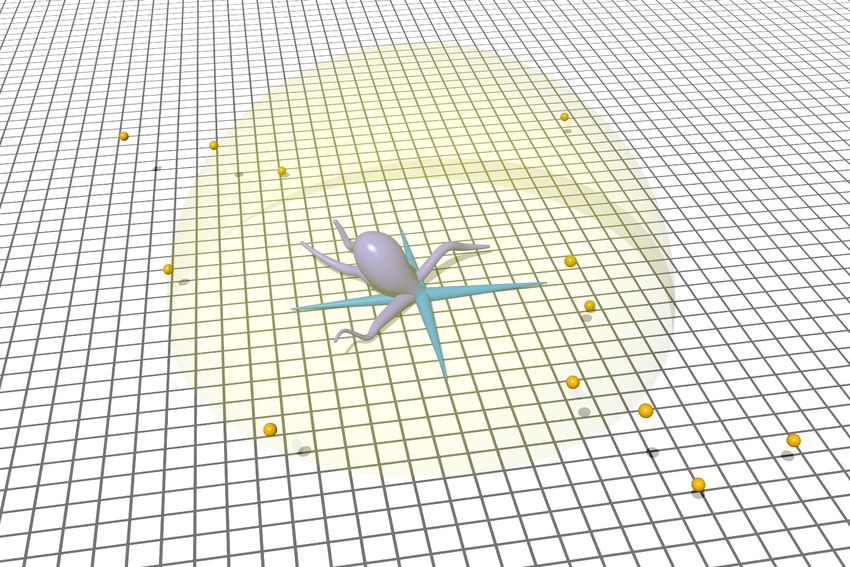
Figure 5: Hierarchical control framework. Based on the locations (relative to the arm base) of targets in the view range, the high-level controller
decides between two actions, crawl or reach all, to maximize gained energy. (a) Demonstration of learned PPO policy for a single active arm as
implemented in Elastica. The active arm is depicted in blue, with the levels of shading indicating intermediate configurations. The CyberOctopus
successfully moves forward and collects available food. Here, F = 5, γ = 5, and Φ = 1.0. A video of this demonstration is available (SI Video 1). (b)
Learning curve of the PPO algorithm for a single active arm. (c) Key metrics for evaluating the performance of hierarchical and end-to-end (e2e)
control schemes. Orange lines represent the metric’s median value, boxes represent the inter-quartile (middle 50%) range, and whiskers denote the
min and max of 100 evaluation samples. PPO is the reinforcement learning algorithm, Q is the analytic solution of a simplified DP problem (see SI
for details), the greedy policy chooses to reach anytime there is food within reach, else it crawls, and the random policy chooses actions randomly.
The e2e approach attempts to directly solve the end-to-end problem (see SI for details). Hierarchy-based control policies are found to outperform
end-to-end solutions, with PPO performing best overall.
simplifying assumptions. After showing favorable comparison between learning-based and analytical solutions,
in Sec. 5.2 we expand our approach to the case of multiple active arms (up to four), for which no analytical
solutions exist. Finally, a third (lowest) level of control based on local physical compliance is incorporated, and a
CyberOctopus outfitted with this tri-level hierarchy is shown to forage in an arena littered with obstacles in 3D
space.
5.1 Foraging with one arm
Analytical solution. As mentioned aboved, there is no analytical solution to the high-level problem of Eq. 13.
However, under simplifying assumptions, analytical solutions may be obtained for the case of a single arm (I = 1).
Here, we make the following assumptions: (1) The workspace W is treated as a rectangle whose width is larger
than the distance the arm can crawl in one step; (2) The energetic cost of each high-level command is simplified
to be a constant, with no dependence on the NN-ES muscle activations; (3) The food reward γ is greater than the
constant cost to reach a target. Under these assumptions, an analytical Q-policy solution to the optimal dynamic
programming (DP) planning problem of a CyberOctopus foraging with one arm can be derived, as detailed in
the SI. We note that the same procedure can be extended to two arms crawling and reaching in two orthogonal
planes (SI). However, if more than two arms are considered, the number of steps to reach all food targets can
not be determined, making the derivation of an optimal analytical policy not possible, even under the above
10simplifying assumptions. However, despite their limited scope, one- and two-arm analytical solutions are still
useful to benchmark and contextualize our hierarchical approach and its learning-based solution, as we progress to
the more general, non-analytically tractable scenario of larger numbers of engaged arms.
Reinforcement Learning solution. We proceed with solving the problem of Eqs. 11-16 for one arm, via the
PPO reinforcement learning algorithm, using the setup described in Section 4.3. The performance of the one-arm
policy, numerically obtained with PPO and dynamically executed by the CyberOctopus in Elastica, is shown in
Figure 5a, while policy convergence during training is illustrated in Fig. 5b. The policy is trained for 2000 epochs,
each epoch entailing 1024 time steps. At the beginning of each episode, 20 targets are randomly generated in a
rectangular area within the arm’s bending plane (Fig. 1b), and the arm is initialized in a straight configuration on
the left side of the food (Fig. 5a). An episode terminates when either all targets have been reached or the number
of time steps exceeds 180, so that each epoch contains at least 5 episodes.
The CyberOctopus (whose only active arm is depicted in blue) successfully learns to crawl towards food, posi-
tioning itself for reaching until all food in the environment is collected (Fig. 5a and SI Video 1). To contextualize
this performance, we implement three alternative high-level controllers: the simplified, analytical Q-policy solution
described above, a ‘greedy’ controller that immediately reaches for food whenever available, otherwise it chooses
to crawl, and a random controller that selects crawl or reach all with equal probability at each time step. We
evaluate the performance of these four controllers on three metrics (Fig. 5c): (1) net energy (Eq. 13), (2) average
number of time steps per food item collected, and (3) average number of crawl steps per food target. We find,
unsurprisingly, that the random policy performs the worst, utilizing, on average, 25% more energy and 40% more
steps per episode than the other approaches. The greedy and Q-policy controllers perform comparably, though the
Q-policy presents a wider distribution than greedy, likely due to simplifying assumptions that cause the occasional
miss of a target. Overall, the PPO policy exhibits the best performance, strategically crawling until a large number
of food items are simultaneously within reach, to then fetch them all at once. In light of the energy cost maps of
Fig. 3d, this learned approach intuitively correlates to lower muscle activation costs. This strategy (which is also
adopted by the Q-policy in the simplified setting of the problem) not only reduces energy costs but additionally
allows completion of the foraging task in a fewer number of time steps (Fig. 5c). As we will see, the performance
gap between PPO and the alternative approaches will only widen as more complex scenarios (I > 1) are considered,
until becoming the only reliable option.
To comparatively isolate the benefits provided by our hierarchical decomposition, we solve the same foraging
problem in an end-to-end (e2e) fashion, using PPO. In other words, we train a single network to directly map food
locations and current muscle activations to output muscle activations, completely bypassing the decomposition
between high-level planning and low-level execution. A comparison between the two approaches is schematically
illustrated through the block diagrams of Fig. 4b,c, with further mathematical and implementation details available
in the SI. We note that while the previous activation α[n̂ − 1] is used by the low-level controller in Fig. 4b, in the
end-to-end formulation depicted in Fig. 4c, this information is included in the state representation. Thus, overall,
the same amount of information is provided to both frameworks.
We find that all four hierarchical policies (including the random policy) outperform the end-to-end approach,
across all metrics (Fig. 5c), despite significant effort in tuning training parameters. This result underscores how
the separation of concerns enabled by the hierarchy significantly simplifies control, and thus learning. Further, it
illustrates the potential of a mixed-modes approach, where model-free and model-based algorithms are employed
at different levels so as to synergize and complement each other.
5.2 Foraging with multiple arms
We next gradually increase the number of active arms engaged by the CyberOctopus, considering first two arms
and then four arms. As the number of arms increases, the CyberOctopus is able to access additional directions
of movement and must coordinate its arm’s behaviors, significantly increasing the problem difficulty. Additionally,
in the four-arm case, we incorporate obstacles into the arena, requiring the arms to exploit their mechanical
intelligence to avoid becoming obstructed.
Foraging with two arms. We first consider a CyberOctopus with two active arms (I = 2), orthogonal
to each other. Training proceeds as with the single arm, although now 10,000 epochs are used. For each episode,
arms are initialized at rest and 20 food locations are scattered randomly throughout the arena on vertical planes
that align with the grid formed by discrete crawling steps. As reported in Fig. 6, the learning-based approach
11(a) Demonstration (b) Performance
1.
Total gained energy
2. 3.
1. Reach with one arm 2. Collect two targets with one arm
and crawl with the other
PPO Q Greedy Random
per targets eaten
# of steps
3. Reach with both arms
PPO Q Greedy Random
Figure 6: (a) Demonstration in Elastica of learning-based PPO policy controlling two arms to forage. (a1) The arms coordinate their actions to
move across two dimensions and reach targets. (a2) One arm collects multiple targets within its bending plane. (a3) Two arms simultaneously
collect targets in their respective bending planes. A video of this demonstration is available (SI Video 2). (b) Performance of the different control
schemes. Orange lines represent the metric’s median value, boxes represent the inter-quartile (middle 50%) range, and whiskers denote the min and
max of 100 evaluation samples. The learning-based PPO policy gains more total energy and requires fewer steps per collected target than the
alternative high-level policies. For the learning-based policy, F = 10.
successfully learns and converges (see SI for learning curves). This is reflected in the evaluation of the corresponding
policies in Fig. 6b. The behavior learned via the learning-based approach is illustrated in Fig. 6a as well as
in SI Video 2. As can be seen, the CyberOctopus crawls between targets and collects them, with the learned
policy successfully coordinating its two independent arms so as to crawl and switch along orthogonal directions,
simultaneously grabbing food with both arms or fetching food with one arm while crawling with the other arm. We
again contextualize our results by means of three alternative high-level controllers: Q is the analytically identified
solution of the simplified DP problem described above and in the SI, greedy has each arm collecting food when
immediately available, else crawling (SI for details), and random selects crawl or reach all with equal probability
for each arm. Again the learning-based solution outperforms the alternative high-level controllers, consistently
collecting more energy and using fewer steps to do so (Fig. 6b). We forego a comparison with the end-to-end
approach, as its performance is deemed too poor to provide any useful insight. This once again underscores the
significant impact of hierarchically decomposing the problem, which in this example amounts to being able to solve
the problem versus not being able to do so (end-to-end).
Foraging with four arms and in the presence of solid obstacles. Having established the viability of our
multi-arm approach, we now consider the problem of a CyberOctopus foraging with four active arms (I = 4). The
arms, being orthogonal to each other, allow the CyberOctopus to fully traverse the substrate by crawling along the
four cardinal directions, rendering the foraging problem analytically intractable. Further, this time, not only food
but also solid obstacles will be distributed in 3D space (Fig. 7a). The goal of this test is two-folds: first we wish
to characterize the ability of out methods to learn to solve this foraging scenario (without obstacles), and second
we wish to explore how principles of mechanical intelligence [31, 58] may be used to deal with such disturbances
(obstacles), without further burdening control or training.
To this end, we incorporate a simple behavioral reflex based on traveling waves of muscle activation observed in
the octopus [46, 47]. When contact between an arm and an obstacle is sensed, two waves emanate from the point
of contact in each direction. One, traveling towards the arm’s tip, signals all muscles to relax, while the second,
traveling towards the arm’s base, signals longitudinal muscles on the contacting side to increase activation with all
other muscles relaxing. Here, we treat these waves as propagating instantaneously. Once contact ceases, the arm
returns to executing the originally prescribed muscle activations. As can be seen in Fig. 7a, this reflex, mediated
by the compliant nature of the arm, allows it to slip past obstacles, thus dealing with their presence with minimal
additional computational effort. On the other hand, without the reflex, the arm routinely gets stuck (Fig. 7c).
12(a) (b)
No local feedback Local feedback
Reaching rate (%)
Drop
75 %
Improve
Stuck Slide past ~2x Recover
50 %
Greedy PPO PPO PPO
( no
)(
obstacles
no
obstacles ) ( no
reflex ) (reflex
with
)
(c) Overcome 0/11 obstacle Overcome 9/11 obstacle 1. Stuck
1. 2.
2. Collect 3 targets
Obstacle
Figure 7: (a) Demonstration of an arm sliding past an obstacle when equipped with local sensory feedback. (b) Percentage of available food items
collected from the environment by the greedy policy (yellow) and the learning-based policy when no obstacles are present (purple), when the arm
does not utilize a reflexive behavior (green), and when the reflex is engaged (blue). Orange lines represent the median performance over 100 episodes,
boxes represent the inter-quartile (middle 50%) range, and whiskers denote the min and max. (c) Demonstration of a foraging CyberOctopus with
four active arms (blue). Using the local sensory reflex allows the arms to overcome 9 of the 11 obstacles that otherwise would cause the arm to
become stuck. (c1) The arms coordinate their actions to move across two dimensions and reach targets. (c2) One arm collects multiple targets
within its bending plane. A video of this demonstration is available (SI Video 3).
The CyberOctopus is then initialized in the center of an arena with 40 food items randomly distributed in 3D
space. Training proceeds without obstacles using the same process of the two-arm case with the learning-based
approach successfully learning to forage. In contrast to the two-arm case, here the CyberOctopus’ four active arms
enable forwards/backwards and left/right crawling, allowing the collection of previously missed food, at a later
stage. This additional freedom increases the planning required to efficiently move throughout the area, not only
making an analytical Q-policy impossible to define, but also substantially impairing the ability of the greedy policy
to collect food. The greedy policy, which is here extended to deal with the case of no targets being in the workspace
(see SI for details), is only able to collect 38% of the food in the arena when engaging four arms, a notable decrease
from the 54% of food collected with two arms. Similarly to the end-to-end approach with two arms, we forgo
a comparison with the random policy here, due to its substantially inferior performance. In contrast, the PPO
learning-based approach is able to successfully exploit this additional freedom (four cardinal directions of motion)
to improve food collection, fetching on average 88% of the food compared to 66% when only two arms are active
(Fig. 7c). The learning-based policy (trained without obstacles) is then deployed in an environment littered with
unmovable obstacles leading to arms becoming stuck, substantially impairing foraging behavior, which now only
achieves 21% food collection. With the sensory reflex enabled, however, the CyberOctopus successfully recovers.
Figure 7c shows the CyberOctopus utilizing this reflexive behavior to reach previously obstructed food (SI Video
3), resulting in 67% of food collected.
6 Conclusion
Recognizing the need for improved control methods in multi-arm soft robots, we propose a hierarchical framework
inspired by the organization of the octopus neurophysiology and demonstrate it in a CyberOctopus foraging for
food. By decomposing control into high-level decision-making, low-level motor activation, and reflexive modulation
via local sensory feedback and mechanical compliance, we show significant improvements relative to end-to-end
approaches. Performance is enabled via a mixed-modes approach, whereby complementary control schemes can
be swapped out at any level of the hierarchy. Here, we combine model-free reinforcement learning, for high-
level decision-making, and model-based energy shaping control, for low-level muscle recruitment and activation.
To enable compatibility in terms of computational costs, we developed a novel, neural-network energy shaping
13(NN-ES) controller that accurately executes arm motor programs, such as reaching for food or crawling, while
exhibiting time-to-solutions more than 200x faster than previous attempts [25]. Our hierarchical approach is
successfully deployed in increasingly challenging foraging scenarios, entailing two- and three-dimensional settings,
solid obstacles, and multiple arms.
Overall, this work presents a framework to explore the control of multiple, compliant and distributed arms,
in both engineering and biological settings, with the latter providing insights and hypotheses for computational
corroboration. We have begun to take initial steps in this regard, testing how principles of mechanical intelligence
and muscle waves of activation [46, 47] may be couched into local reflexive schemes for accommodating solid
obstacles. Future work will build on these foundations, exploring how distributed control approaches might enable
more biologically plausible manners [31] or how principles of mechanical intelligence may be further extended.
Data Access
The open-source Python implementation of Elastica is available at www.github.com/GazzolaLab/PyElastica. All
codes used in this paper are available at https://github.com/chshih2/Real-time-control-of-an-octopus-a
rm-NNES and https://github.com/chshih2/Multi-arm-coordination-for-foraging.
Supporting Information
Supporting information is available from the authors upon request.
Acknowledgements
We gratefully acknowledge Tigran Norekian and Ekaterina D. Gribkova who performed the histology of the octopus
arm in Figure 2a. This study was jointly funded by ONR MURI N00014-19-1-2373 (M.G., P.G.M.), ONR N00014-
22-1-2569 (M.G.), NSF EFRI C3 SoRo #1830881 (M.G.), and with computational support provided by the Bridges2
supercomputer at the Pittsburgh Supercomputing Center through allocation TG-MCB190004 from the Extreme
Science and Engineering Discovery Environment (XSEDE; NSF grant ACI-1548562).
References
[1] A. Sadeghi, A. Mondini, B. Mazzolai, Soft Robotics 2017, 4, 3 211.
[2] X. Zhang, F. Chan, T. Parthasarathy, M. Gazzola, Nature Communications 2019, 10, 1 1.
[3] H. Huang, F. Uslu, P. Katsamba, E. Lauga, M. Sakar, B. Nelson, Science advances 2019, 5, 1 eaau1532.
[4] C. Della Santina, C. Duriez, D. Rus, arXiv preprint arXiv:2110.01358 2021, 1–69.
[5] T. George Thuruthel, Y. Ansari, E. Falotico, C. Laschi, Soft Robotics 2018, 5, 2 149.
[6] D. Trivedi, C. Rahn, W. Kier, I. Walker, Applied Bionics and Biomechanics 2008, 5, 3 99.
[7] M. W. Hannan, I. D. Walker, Advanced Robotics 2001, 15, 8 847.
[8] M. Baumgartner, F. Hartmann, M. Drack, D. Preninger, D. Wirthl, R. Gerstmayr, L. Lehner, G. Mao,
R. Pruckner, S. Demchyshyn, et al., Nature materials 2020, 19, 10 1102.
[9] A. C. Noel, D. L. Hu, Journal of Experimental Biology 2018, 221, 7 jeb176289.
[10] X. Lu, W. Xu, X. Li, In 2015 6th international conference on automation, robotics and applications (ICARA).
IEEE, 2015 332–336.
[11] E. B. Joyee, Y. Pan, Soft robotics 2019, 6, 3 333.
[12] B. Gamus, L. Salem, A. D. Gat, Y. Or, IEEE Robotics and Automation Letters 2020, 5, 2 1397.
[13] P. Karipoth, A. Christou, A. Pullanchiyodan, R. Dahiya, Advanced Intelligent Systems 2022, 4, 2 2100092.
[14] I. Must, E. Sinibaldi, B. Mazzolai, Nature communications 2019, 10, 1 1.
[15] J. M. Skotheim, L. Mahadevan, Science 2005, 308, 5726 1308.
14[16] M. Otake, Y. Kagami, M. Inaba, H. Inoue, Robotics and Autonomous Systems 2002, 40, 2-3 185.
[17] H. Jin, E. Dong, G. Alici, S. Mao, X. Min, C. Liu, K. Low, J. Yang, Bioinspiration & biomimetics 2016, 11,
5 056012.
[18] X. Zhang, N. Naughton, T. Parthasarathy, M. Gazzola, Nature Communications 2021, 12, 1 6076.
[19] H. Marvi, C. Gong, N. Gravish, H. Astley, M. Travers, J. Hatton, R.L.and Mendelson, H. Choset, D. Hu,
D. Goldman, Science 2014, 346, 6206 224.
[20] T. Li, K. Nakajima, M. Calisti, C. Laschi, R. Pfeifer, 2012 IEEE International Conference on Mechatronics
and Automation, ICMA 2012 2012, 948–955.
[21] M. Cianchetti, M. Calisti, L. Margheri, M. Kuba, C. Laschi, Bioinspiration and Biomimetics 2015, 10, 3.
[22] M. D. Grissom, V. Chitrakaran, D. Dienno, M. Csencits, M. Pritts, B. Jones, W. McMahan, D. Dawson,
C. Rahn, I. Walker, Unmanned Systems Technology VIII 2006, 6230, May 2006 62301F.
[23] Q. Wu, X. Yang, Y. Wu, Z. Zhou, J. Wang, B. Zhang, Y. Luo, S. A. Chepinskiy, A. A. Zhilenkov, Bioinspiration
& Biomimetics 2021, 16, 4 046007.
[24] Y. Sakuhara, H. Shimizu, K. Ito, In 2020 IEEE 10th International Conference on Intelligent Systems (IS).
IEEE, 2020 463–468.
[25] H.-S. Chang, U. Halder, E. Gribkova, A. Tekinalp, N. Naughton, M. Gazzola, P. G. Mehta, In 2021 60th IEEE
Conference on Decision and Control (CDC). IEEE, 2021 1383–1390.
[26] J. Walker, C. Ghalambor, O. Griset, D. McKenney, D. Reznick, Functional Ecology 2005, 19, 5 808.
[27] F. Grasso, American Malacological Bulletin 2008, 24, 1 13.
[28] E. Kennedy, K. C. Buresch, P. Boinapally, R. T. Hanlon, Scientific reports 2020, 10, 1 1.
[29] P. Godfrey-Smith, Scientific American Mind 2017, 28, 1 62.
[30] J. Young, Journal of anatomy 1971, 112 144.
[31] B. Hochner, Current Biology 2012, 22, 20 R887.
[32] G. Sumbre, Y. Gutfreund, G. Fiorito, T. Flash, B. Hochner, Science 2001, 293, 5536 1845.
[33] T. Hague, M. Florini, P. L. Andrews, Journal of experimental marine biology and ecology 2013, 447 100.
[34] T. Gutnick, L. Zullo, B. Hochner, M. J. Kuba, Current Biology 2020, 30, 21 4322.
[35] H.-S. Chang, U. Halder, C.-H. Shih, A. Tekinalp, T. Parthasarathy, E. Gribkova, G. Chowdhary, R. Gillette,
M. Gazzola, P. G. Mehta, In 2020 59th IEEE Conference on Decision and Control (CDC). IEEE, 2020
3913–3920.
[36] M. Gazzola, L. H. Dudte, A. G. McCormick, L. Mahadevan, Royal Society Open Science 2018, 5, 6.
[37] W. Kier, M. Stella, Journal of Morphology 2007, 268, 10 831.
[38] S. S. Antman, Nonlinear Problems of Elasticity, Springer, 1995.
[39] B. Zhang, Y. Fan, P. Yang, T. Cao, H. Liao, Soft Robotics 2019, 6, 3 399.
[40] N. Naughton, J. Sun, A. Tekinalp, T. Parthasarathy, G. Chowdhary, M. Gazzola, IEEE Robotics and Automa-
tion Letters 2021, 6, 2 3389.
[41] O. Aydin, X. Zhang, S. Nuethong, G. Pagan-Diaz, R. Bashir, M. Gazzola, M. Saif, Proceedings of the National
Academy of Sciences 2019, 116, 40 19841.
[42] G. Pagan-Diaz, X. Zhang, L. Grant, Y. Kim, O. Aydin, C. Cvetkovic, E. Ko, E. Solomon, J. Hollis, H. Kong,
T. Saif, M. Gazzola, R. Bashir, Advanced Functional Materials 2018, 28, 23 1801145.
[43] J. Wang, X. Zhang, J. Park, I. Park, E. Kilicarslan, Y. Kim, Z. Dou, R. Bashir, M. Gazzola, Advanced
Intelligent Systems 2021, 2000237.
15You can also read