Human Reidentification with Transferred Metric Learning
←
→
Page content transcription
If your browser does not render page correctly, please read the page content below
Human Reidentification
             with Transferred Metric Learning

                      Wei Li, Rui Zhao and Xiaogang Wang

     Electronic Engineering Department, the Chinese University of Hong Kong

       Abstract. Human reidentification is to match persons observed in non-
       overlapping camera views with visual features for inter-camera tracking.
       The ambiguity increases with the number of candidates to be distin-
       guished. Simple temporal reasoning can simplify the problem by prun-
       ing the candidate set to be matched. Existing approaches adopt a fixed
       metric for matching all the subjects. Our approach is motivated by the
       insight that different visual metrics should be optimally learned for dif-
       ferent candidate sets. We tackle this problem under a transfer learning
       framework. Given a large training set, the training samples are selected
       and reweighted according to their visual similarities with the query sam-
       ple and its candidate set. A weighted maximum margin metric is online
       learned and transferred from a generic metric to a candidate-set-specific
       metric. The whole online reweighting and learning process takes less than
       two seconds per candidate set. Experiments on the VIPeR dataset and
       our dataset show that the proposed transferred metric learning signif-
       icantly outperforms directly matching visual features or using a single
       generic metric learned from the whole training set.

1    Introduction
Human reidentification has drawn great interest in video surveillance recently
[1–4]. It is to match humans observed in non-overlapping camera views based
on their visual features and is very important for inter-camera tracking. Human
reidentification is a challenging problem, since the same person observed in dif-
ferent camera views undergoes significant changes of resolutions, lightings, poses
and viewpoints. Because humans captured by surveillance cameras, especially
in far-field video surveillance, are often in small sizes and a lot of their visual
details such as facial components are indistinguishable in images, some of them
look similar in appearance. The ambiguity increases with the number of persons
to be distinguished. Many visual features of characterizing color [5, 6], shape [7, 8]
and texture [9–11] of objects have been proposed. In order to overcome the large
visual changes across camera views, learning approaches were typically adopted.
They learned either the transformations of visual features between camera views
[12–15] or visual distance metrics [16–18, 2, 19, 4] from a training set.
    In inter-camera tracking, given a query sample observed in a camera view,
simple temporal reasoning can be made by roughly estimating the transition time
across cameras. Such reasoning can simplify the matching problem by pruning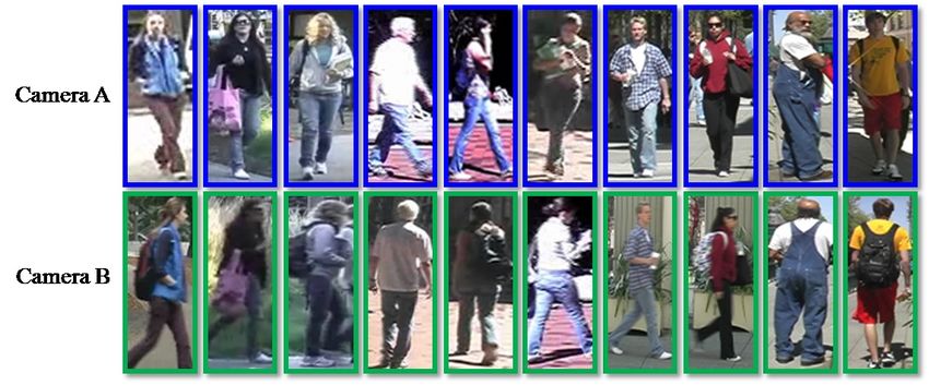
2       Wei Li, Rui Zhao, Xiaogang Wang

                    (a)                                        (b)

Fig. 1. Examples of query samples and their corresponding candidate sets in human
reidentification. (a1) and (b1) are query samples observed in a camera view. (a2) and
(b2) are persons in the corresponding candidate sets observed in another camera view
after pruning with temporal reasoning. The red windows indicate the truly matched
persons. The persons in candidate set (a2) can be well distinguished with color his-
tograms but some of them have similar texture. The persons in candidate set (b2) have
similar color histograms. Therefore, distinguishing them has to rely more on other type
of features.

the candidate set observed in another camera view. Existing approaches always
use the same set of visual features and a fixed distance metric to match any
query samples with any candidates, which is not an optimal solution. Since the
goal is to distinguish a small number of persons in a particular candidate set, a
candidate-set-specific visual metric is preferred. As an example shown in Figure
1, the persons in the first candidate set can be well distinguished with color his-
tograms, while those in the second candidate set are similar in color and other
features such as shape and texture could be more effective on them. Unfortu-
nately, each person in the candidate set only has one sample observed in one
camera view since the correspondences of samples across camera views are un-
known during online tracking, while metric learning requires pairs of samples
observed in different camera views with correspondence information. Therefore,
directly applying existing metric learning algorithms to obtain a candidate-set-
specific metric is infeasible. We tackle this problem under a transfer learning
framework. As shown in Figure 2, for each sample in the candidate set, its near-
est neighbors in the training set are found by directly matching their visual
features. When the training set is large, the found nearest neighbors are likely
to be visually similar to the sample in the candidate set and their corresponding
training samples in another camera view are known with the ground truth la-
bels. Therefore, the candidate-set-specific metric can be indirectly learned from
the selected training pairs. These training pairs are weighted according to their
visual similarities to the samples in the candidate set and the query sample.
For each candidate set, a metric which maximizes the margin between the cor-
rectly matched pairs and wrongly matched pairs is learned [20]. In order to avoid
overfitting, the candidate-set-specific metric is regularized by a generic metric
learned from the whole training set. To the best of our knowledge, this is the
first time for transfer learning to be applied to human reidentification. Exper-
iments on the VIPeR database [21] and our dataset show that it significantly
outperforms the approach of directly matching visual features or using a generic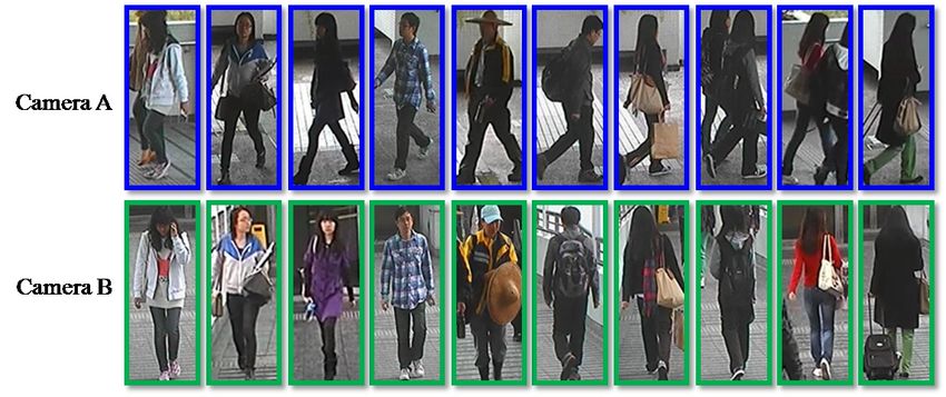
Human Reidentification with Transferred Metric Learning 3
distance metric. The weighting and transfer learning process takes less than two
seconds per candidate set. It can be applied to both online and offline human
reidentification.
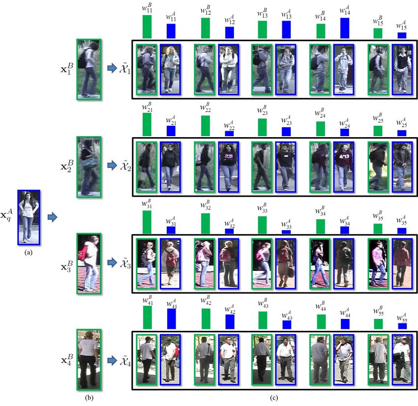
Fig. 2. (a) A query sample observed in camera view A. (b) Samples of four candidate
persons observed in camera B based on temporal reasoning. (c) The nearest neighbors
of each candidate in (b) found from a large training set by directly matching the
visual features observed in camera B. Each person in the training set has a pair of
samples observed in both cameras A and B according to manually labeled ground
truth. Therefore the paired samples of the found nearest neighbors can be used to train
the candidate-set-specific metric. Blue windows indicate samples observed in camera A
A B
and green windows indicate samples observed in camera B. wij and wij are the weights
assigned to training samples according to their visual similarities with the candidates
and the query sample respectively. See details in Section 3.2.
2 Related Work
Many approaches have been proposed to learn the distance metrics to match the
visual features of image regions observed in different camera views. Schwartz
and Davis [2] proposed an approach of projecting high dimensional features to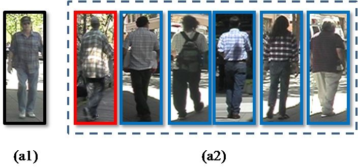
4       Wei Li, Rui Zhao, Xiaogang Wang

a low dimensional discriminant latent space by Partial Least Squares reduction.
It weighted features according to their discriminative power to best distinguish
the observations of one object with those of others in the training set in a one-
against-all scheme. Lin and Davis [18] learned a different pairwise dissimilarity
profile which best distinguished a pair of persons. It was assumed that a feature
may be crucial to discriminate two very similar objects but not be effective
for other objects. Therefore it is easier to train discriminative features in a
pairwise scheme. However, these two approaches required that all the persons to
be reidentified have examples in the training set. They can not re-identify a new
person. Zheng et al. [4] proposed a Probabilistic Relative Distance Comparison
model. It formulated object reidentification as a distance learning problem and
maximized the probability that a pair of true match has a smaller distance than
a wrong match pair. In [16, 19] boosting and RankSVM were used to select an
optimal subset of features for matching objects across camera views. They could
be generalized to persons outside the training set. They targeted on learning a
generic metric to distinguish all the persons, which is very challenging since the
distribution of visual features from arbitrary persons is very complex. Moreover,
any generic metric could be suboptimal for a specific subset of persons whose
visual features distribute in some local regions of the high dimensional feature
space.
    Transfer learning assumes that the distribution of the training data differs
from the test data. It automatically adjusts the weights of training samples to
match the distributions of training and test data. Various transfer learning algo-
rithms, such as TrAdaBoost [22], weighted margin SVM [23], localized SVM [24]
and cross-domain SVM [24] were proposed. Transfer learning has been widely
applied to various vision problems such as object recognition [25], object detec-
tion [26], image and video retrieval [27], and visual concept classification [28, 24,
29, 30]. In cross-domain SVM [24], each training sample is weighted according
to its closeness to the test data. It is related to our approach. However, different
than [24], a distance metric instead of a hyperplane is learned in our case. Besides
reweighting training samples, our adaptive metric is also regularized by a generic
metric. Query-specific distance metric learning [31] optimally distinguishes query
person with anyone else in the dataset, while ours optimally distinguish query
person with others ONLY in the candidate set. So ours is both query-specific
and candidate-set-specific which is the most important novelty of this paper.

3     Our Method
3.1   Visual Features
We employ five types of low-level visual features including dense color his-
tograms, dense SIFT [32], HOG [7], Gabor [24] and LBP [10]. They charac-
terize the color distributions, shape and texture of objects. Image regions are
normalized to 160 × 60. For dense color histograms and dense SIFT, a uniform
20 × 12 grid is placed on the image region, and color histograms in the RGB
color space and SIFT descriptors are densely computed on the grid. For each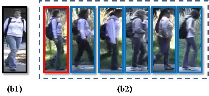
Human Reidentification with Transferred Metric Learning                  5

type of features, PCA is applied to retain 90% energy and then each feature
vector is normalized to zero mean and unit variance. Different types of features
are concatenated to form a single feature vector.

3.2    Searching and weighting training samples
Our approach includes two key steps: searching and weighting nearest training
samples for each candidate; and learning an adaptive metric for each candidate
set. Let xA     q be the visual feature vector of a query sample observed in camera A,
and XcB = {xB                      B
                      1 , . . . , xN } be a set of candidates observed in camera view B after
pruning with temporal reasoning. For each candidate xB                                        B
                                                                      i , a set of samples X̃i =
{x̃B
   i1 , . . . , x̃ B
                   iK } close     to x B
                                       i is selected from the training set  S. A  straightforward
               i

way is to set X̃iB as the K nearest neighbors of xB                          B
                                                  i in S (denoted with NK (xi ))
by comparing the visual features. However, this approach is not quite stable,
since some xB i may be dissimilar with any samples in S. In that case, none of
the training samples should be selected and we should rely on the generic metric.
We recompute the similarity between xB                     B
                                         i and a sample x̃j in S as following,

                                            |NK (xB           B
                                                  i ) ∩ NK (x̃j )|
                           s(xB     B
                              i , x̃j ) =                          .                         (1)
                                            |NK (xB           B
                                                  i ) ∪ NK (x̃j )|

The intuition is that if xB                           B
                                         i and x̃j are visually similar, they should share
more nearest neighbors in the training set1 . X̃iB is selected by choosing x̃B                j
with s(xB       B
          i , x̃j ) > s0 , where s0 is a threshold. NK (·) characterizes the geomet-
ric structures of the training set. It is more reliable than directly thresholding
the visual distance kxB                    B 2
                               i − x̃j k2 , whose value is difficult to be interpreted and
whose threshold is hard to be decided. The nearest neighbors of training sam-
ples can be pre-computed offline and a reverse mapping maintains the neighbors
of each sample. After NK (xB              i ) is online efficiently computed with Approximate
Nearest Neighbor Search [33], s(xB                      B
                                                  i , x̃j ) can be computed with a complexity of
O(K) using the reverse mapping. Once X̃iB is chosen, the corresponding training
pairs X̃i = {(x̃A         B                A       B
                   i1 , x̃i1 ), . . . , (x̃iKi , x̃iKi )} are obtained since the correspondences
of training samples are known. In practice, one training sample x̃B                 j may corre-
spond to multiple training samples in camera view A and more training pairs
are obtained. In order to simplify the description, we assume that x̃B                j only has
one corresponding sample in another camera view without affecting the gener-
alization of the proposed algorithm.
    Each training pair (x̃A                 B
                                     ij , x̃ij ) is assigned with a weight wij according to its
visual similarities with the candidate sample xB                                           A
                                                                  i and the query sample xq . A
training pair with a larger weight will have larger contribution for learning the
adaptive metric. wij is defined as following,
                                              B     A
                                       wij = wij · wij ,                                     (2)
1
    In our implementation K = 10.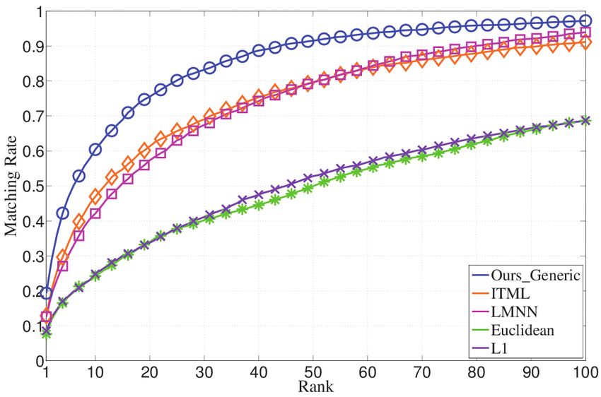
6       Wei Li, Rui Zhao, Xiaogang Wang
                                                                      !
                              B
                                                      kxB     B 2
                                                        i − x̃ij k2
                             wij       = exp −                            ,              (3)
                                                          2σi2
                                                                      !
                              A
                                                      kxA     A 2
                                                        q − x̃ij k2
                             wij = exp −                                  ,              (4)
                                                          2σ02
where σi2 = median({kxB    B 2                     2              A    A 2
                      i −x̃ij k2 }x̃B ∈X̃ B ) and σ0 = median({kx̃i −x̃j k2 }x̃A    A
                                                                               i ,x̃j ∈S
                                                                                         ).
                                            ij    i
  B
wij  is straightforward, since the selected training samples are supposed to be vi-
                                       A
sually similar to the candidates. wij    has two purposes. (1) Even though some
selected samples are similar with the candidate in camera B, their samples ob-
served in camera A may be dissimilar with the query sample, because of pose
variations. It is not useful to learn the adaptive metric from such training pairs,
since their inter-camera variations are different than that of the query person.
The learned adaptive metric is supposed to depress the inter-camera variation
of the query person. (2) If the selected training samples are similar to xq in
camera A, their corresponding candidate persons are easy to be confused with
the query person. Therefore, we should give more weights to their training sam-
ples to well distinguish them in transfer learning. Some examples are shown in
               A
Figure 2. {w2j   } of the samples in X̃2 are low because their observations in A
have very different colors than the query sample and the second candidate can
                                                       A
be easily distinguished from the query person. {w3j      } of the samples in X̃3 are
also low because their pose variations are different than that of the query per-
son. The inter-camera variation of the query person is not well captured by the
                                    A           A
training samples in X̃3 . Both {w1j   } and {w4j  } have large weights because the
first and the fourth candidates are similar to the query person and therefore a
metric needs to be specially trained to extract their subtle differences. Also the
inter-camera variations existing in X̃1 and X̃4 well match with that of the query
person.

3.3   Learning adaptive metrics by maximizing weighted margins
Given a positive semidefinite (PSD) matrix M , the distance between two samples
xA       B
 i and xj observed in two different camera views is computed as

                        d(xA    B       A    B t     A    B
                           i , xj ) = (xi − xj ) M (xi − xj ).                           (5)
   We first learn a generic metric M0 from the whole training set S. Given a
query sample xq , its candidate set XcB and the selected training pairs {X̃i }N
                                                                              i=1 ,
an adaptive metric M is learned with a regularization added by M0 . It minimizes
the following objective function with constraints,
                                  X
           min kM − M0 k2F + C        wij · wi0 j 0 · ξiji0 j 0 ,              (6)
            s.t. (x̃A      B t         A      B           A      B t       A      B
                    ij − x̃i0 0 ) M (x̃ij − x̃i0 0 ) − (x̃ij − x̃ij ) M (x̃ij − x̃ij )
                             j                        j

                  ≥1−ξ      iji0 j 0     ∀i, j, i , j 0 , i 6= i0
                                                  0
                                                                                         (7)
                  M  0, ξiji0 j 0 ≥ 0                                                   (8)
Human Reidentification with Transferred Metric Learning 7
Algorithm 1: Learning an adaptive metric for each candidate set by op-
timizing (6-8) with the cutting plane method.
1 W = ∅;
2 M = M0 ;
3 ξiji0 j 0 = 0;
4 begin
5 repeat
6 (î, ĵ, î0 , ĵ 0 ) = arg max wij · wi0 j 0 (1 − ψiji0 j 0 (M ));
(i,j,i0 ,j 0 )
7 if 1 − ψîĵ î0 ĵ 0 (M ) > ξîĵ î0 ĵ 0 + then
8 W = W ∪ {(î, ĵ, î0 , ĵ 0 )};
9 Solve the following QP problem using ADMM;
(M, {ξiji0 j 0 }) = arg min ||M − M0 ||2F + C iji0 j 0 wij · wi0 j 0 · ξiji0 j 0
P
10
11 s.t. ∀(i, j, i0 , j 0 ) ∈ W
12 (x̃A B t A B A B t A B
ij − x̃i0 0 ) M (x̃ij − x̃i0 0 ) − (x̃ij − x̃ij ) M (x̃ij − x̃ij ) ≥ 1 − ξiji0 j 0
j j
13 M 0, ξiji0 j 0 ≥ 0
14 until W does not change;
The distance between two metrics is define as
X
kM − M0 k2F = (M [i, j] − M0 [i, j])2 = tr((M − M0 )(M − M0 )t ). (9)
ij
(x̃A B t A B
ij − x̃ij ) M (x̃ij − x̃ij ) is the distance between two samples of the same person
(i, j) observed in different camera views under the metric M . It is supposed to
be smaller than any (x̃A B t A B
ij − x̃i0 0 ) M (x̃ij − x̃i0 0 ), which is the distance between
j j
the samples of (i, j) and a different person (i0 , j 0 ), with a margin. The slack
penalties are weighted with wij and wi0 j 0 . Here we require that i 6= i0 . If i = i0 ,
the two selected training persons (i, j) and (i, j 0 ) are actually related to the same
candidate and we do not have to distinguish them.
Our objective function (6) is convex with liner constraints,
ψiji0 j 0 (M ) = (x̃A B t A B A B t A B
ij − x̃i0 0 ) M (x̃ij − x̃i0 0 ) − (x̃ij − x̃ij ) M (x̃ij − x̃ij )
j j
= tr(M (x̃A B A B t A B A B t
ij − x̃i0 0 )(x̃ij − x̃i0 0 ) ) − tr(M (x̃ij − x̃ij )(x̃ij − x̃ij ) )
j j
≥ 1 − ξiji0 j 0 . (10)
It can be solved by Semidefinite Programming (SDP). We did not choose the sub-
gradient method [34], which has been used by many metric learning approaches
[35], to solve this optimization problem, because it simultaneously considers all
the constraints and the computational cost is high. Instead, we adopt the cutting
plane method [36] and our learning steps are summarized in Algorithm (1). Since
M is initialized with M0 which is a reasonably good starting point, only a small
portion of samples violate the constraints of (7) during the optimization process.8 Wei Li, Rui Zhao, Xiaogang Wang
At each of the iterative steps, we choose samples with the largest violation of
the constraint of margin,
(î, ĵ, î0 , ĵ 0 ) = arg max wij · wi0 j 0 (1 − ψiji0 j 0 (M )), (11)
(i,j,i0 ,j 0 )
and add them to a working set W 2 . Then M and {ξiji0 ji } are optimized only
considering the constraints added by the samples in W. The objective function
(6) is quadratic in M and linear in ξiji0 j 0 , and can be solved using Quadratic Pro-
gramming (QP). We implement the QP solver using the Alternating Direction
Method of Multipliers (ADMM) [37]3 which was proven to have a fast conver-
gence rate. Our optimization procedure is inspired by structural SVM [20] where
the cutting plane method was also used and it converged fast. The convergence
of our algorithm is guaranteed, since W cannot increase forever. The convergence
rate of our algorithm is controlled by and a global optimal with violation of
margin is obtained. Asymptotically, with → 0, the global optimal can be ob-
tained. According to the suggestions of [20], we choose = 0.001. The parameter
C is chosen as 1/mean({kx̃i − x̃j k22 }x̃i ,x̃j ∈S ) referring to the recommendation of
SVMLight4 .
From (2-4) and (6-8) it is observed that if a query sample and its candidate
set are dissimilar with any samples in the training set, few training samples
are selected and their weights are small. In that case, there are few constraints
and the adaptive metric M is very close to generic metric M0 . Learning the
generic metric. M0 is learned by minimizing the following objective function,
X
min kM0 k2F + C ξij ,
i,j
s.t. (x̃A
i − x̃B t A
j ) M0 (x̃i − x̃B A B t A B
j ) − (x̃i − x̃i ) M0 (x̃i − x̃i ) ≥ 1 − ξij , ∀i, j, i 6= j
M0 0, ξiji0 j 0 ≥ 0 (12)
All the samples in the whole training set are included. (x̃A B
i , x̃i ) are the training
samples of the same person observed in different camera views, and (x̃A B
i , x̃j ) are
the training samples of different persons. Once M0 is learned, it is normalized
M0
by M0 = tr(M 0)
.
4 Experimental Results
4.1 Dataset Description
Experiments are conducted on the VIPeR dataset [21] and the Campus 5 dataset
built by us. The VIPeR dataset is a widely used benchmark for evaluating human
2
W is initialized as empty and no samples are removed from W during the optimiza-
tion procedure.
3
In ADMM, after each gradient step, the updated M is projected back onto the
feasible set of PSD matrices by spectral decomposition.
4
http://svmlight.joachims.org/
5
http://www.ee.cuhk.edu.hk/~xgwang/CUHK_identification.htmlHuman Reidentification with Transferred Metric Learning 9
(a) VIPeR
(b) Campus
Fig. 3. Examples of images from the VIPeR dataset and the Campus dataset.
reidentification algorithms. It includes 632 persons captured in two camera views.
Each person has one image per camera view. The Campus dataset has 971
persons and each person also has two images captured in two disjoint camera
views. Some examples of images from the two datasets are shown in Figure
3. Large inter-camera variations are observed in both datasets, which makes
human reidentification challenging. The VIPeR dataset is even more challenging
because even in the same camera view, persons appear in different poses and
viewpoints, and lighting and background also change. It is difficult to learn a
single generic metric to depress many kinds of inter-camera variations. In the
Campus dataset, camera B mainly includes images of the frontal view and the
back view, and camera A has more variations of viewpoints and poses.
4.2 Generic metric learning
We first test our generic metric learning algorithm, i.e., learning M0 by min-
imizing (12), and compare it with other metric learning algorithms and the
state-of-the-art human reidentification algorithms. The accumulative recogni-
tion accuracies on the VIPeR and Campus datasets are shown in Figure 4. For
each of them, 50% persons are randomly selected for training and the remain-
ing ones are used for testing. The random partition is repeated for ten times10 Wei Li, Rui Zhao, Xiaogang Wang
(a) VIPeR (b) Campus
Fig. 4. Evaluate the performance of generic metric learning on the whole gallery set
without using temporal reasoning to prune the candidates. See details in Section 4.2.
and the average accuracies are computed. It is assumed that temporal reasoning
is not used and each query sample matches the object from the whole gallery
set. This is the scenario all the existing human reidentification algorithms as-
sumed. We compare with two state-of-the-art metric learning algorithms, Large
Margin Nearest Neighbor Classification (LMNN) [35] and Information-Theoretic
Metric Learning (ITML) [38], as well as directly matching visual features with
Euclidean distance (Euclidean) and L1 distance (L1 ). Our learned generic metric
(Ours Generic) has a better performance. Its rank-one accuracy is 19.3% on the
VIPeR dataset. Some other state-of-the-art human reidentification techniques
with different visual features and learning algorithms were also evaluated on the
VIPeR dataset and published in literature with the same gallery size and in the
same way of randomly partitioning the dataset [4]. The highest rank one accu-
racy reported so far is 15.66% [4]. Since their implementations are not available,
we do not have their results on the Campus dataset. Compared to PRDC in
[4], our methods enjoy a global optimal solution. Compared with ITML, our
generic metric learning method employs a relative distance comparison rather
than a hard global threshold between negative and positive pairs. For LMNN,
as the distance is measured cross domain, the initial neighborhood selection will
probability have no samples from the same identity selected which will bias the
whole optimization procedure. Our generic metric learning algorithm for human
reidentification is at least comparable with the state-of-the-art. However, this
is not the main contribution of our framework. We focus on transferred metric
learning.
4.3 Transferred metric learning
In this experiment, it is assumed that temporal reasoning can prune candidates
and therefore for each query image the size of the candidate set could be much
smaller than the gallery size. We have tried different sizes (N ) of candidate sets
from 5 to 50. The partitioning of training/test subsets is in the same way as
Section 4.2. We design our experiment to simulate the real world scenario by
random sampling the query-candidate configuration based on the assumptionHuman Reidentification with Transferred Metric Learning 11
(a) VIPeR (b) Campus
Fig. 5. Average accumulative recognition accuracies and their standard deviations on
the candidate sets. The size of the candidate sets is fixed as 15. The bars indicate
standard deviations
that appearance is independent of the temporal reasoning. In order to validate
our approach with a wide variety of configurations, for each query sample in the
test set, we randomly select N −1 samples observed in the other camera view from
the test set and also select the truly matched sample to form its candidate set.
The same experimental design was also adopted in [3]. Human reidentification
is to recognize the right person from the N candidates. For each query image,
this process is repeated for 50 times given a fixed training/test data partition.
The partition of training/test data is repeated for 10 times. When the size of
candidate sets is fixed as 15, the average accumulative recognition accuracies
and their standard deviations on the two datasets are shown in Figure 5. Our
transferred metric learning (Ours Transferred) clearly outperforms our generic
metric learning as well as other generic metric learning algorithms such as ITML
and LMNN. The rank-one accuracy has been improved by 6.32% and 9.71% on
the VIPeR dataset and the Campus dataset respectively. With an unoptimized
matlab implementation and on a Core 8 2.27GHz CPU, it takes less than two
seconds to train an adaptive metric for a candidate set of size 15. Figure 6 plots
the average rank-one accuracies and their standard deviations when the size (N )
of the candidate sets varies from 5 to 50. When N is small, the generic metric
performs well and the improvement of the transferred metric learning is relatively
small. When N is too large (> 50), the distributions of samples in the candidate
set is complicated and close to the global distribution of the whole training set.
In this case, the idea of adapting the metric to a local region of the training set is
not feasible any more and most training samples are selected as the neighbors of
the candidate set. Therefore, the learned adaptive metric is similar to the generic
metric and the improvement becomes little. Compared with figure 4(b) in [3],
the settings are same to ours and our approach outperforms the result test using
the manually designed feature in VIPeR benchmark dataset with all candidate
set size reported in their paper. The size of the training set is an important
factor affecting the effectiveness of transfer learning. When the training set is
large, it is more likely for the candidates to find similar training samples. Figure12 Wei Li, Rui Zhao, Xiaogang Wang
(a) VIPeR (b) Campus
Fig. 6. Average rank-one accuracies when size of candidate sets varies from 5 to 50.
(a) VIPeR (b) Campus
Fig. 7. Average rank-one accuracies when the size of the training set changes.
7 plots the average rank-one accuracies when the size of the training set changes.
When the training set gets large, the difference between the transferred metric
learning and generic metric learning becomes large.
5 Conclusions and Discussions
In this paper, we solve the human reidentification problem from a new angle.
Instead of trying to learn a generic metric to distinguish all the persons and to
depress all types of inter-camera variations, we learn an adaptive metric for a
specific candidate set under the framework of transfer learning. Given a query
sample and its candidate set, the samples in the training set are selected and
reweighted. An adaptive metric is learned by maximizing weighted margin of the
selected training samples and being regularized by a generic metric. Experiments
on the widely used VIPeR dataset and our Campus dataset shows that trans-
ferred metric learning is more effective than generic metric learning on human
reidentification.
In this paper, we assume that the samples are from two fixed camera views.
But the proposed approach also has good potentials to be generalized to the
case when training and testing sets have multiple camera views or even the case
when training and testing data are taken with different cameras. In the VIPeR
dataset, persons captured by the same camera show a large diversity on poses,
viewpoints, lightings and background. It is close to the general case of moreHuman Reidentification with Transferred Metric Learning 13
camera views. In our approach, the training samples are selected and weighted
by matching the visual features with the test samples. Therefore, the selected
training samples should well match the query sample and candidate samples
in pose, viewpoint and lighting even though they may be taken by different
cameras. In the future work, we will build a new dataset with diversified camera
views and will further improve our approach to make it work in more general
camera settings.
6 Acknowledgment
This work is supported by the General Research Fund sponsored by the Research
Grants Council of Hong Kong (project No. CUHK417110 and CUHK417011) and
National Natural Science Foundation of China (project no. 61005057).
References
1. Gheissari, N., Sebastian, T.B., Rittscher, J., Hartley, R.: Person reidentification
using spatiotemporal appearance. In: CVPR. (2006)
2. Schwartz, W., Davis, L.: Learning discriminative appearance-based models using
partial least sqaures. In: Proc. XXII SIBGRAPI. (2009)
3. Farenzena, M., Bazzani, L., Perina, A., Murino, V., Cristani, M.: Person re-
identification by symmetry-driven accumulation of local features. In: CVPR. (2010)
4. Zheng, W., Gong, S., Xiang, T.: Person re-identification by probabilistic relative
distance comparison. In: CVPR. (2011)
5. Park, U., Jain, A., Kitahara, I., Kogure, K., Hagita, N.: Vise: Visual search engine
using multiple networked cameras. In: ICPR. (2006)
6. Weijer, J., Schmid, C.: Coloring local feature extraction. In: ECCV. (2006)
7. Dalal, N., Triggs, B.: Histograms of oriented gradients for human detection. In:
CVPR. (2005)
8. Wang, X., Doretto, G., Sebastian, T., Rittscher, J., Tu, P.: Shape and appearance
context modeling. In: ICCV. (2007)
9. Daugman, J.G.: Uncertainty relation for resolution in space, spatial frequency,
and orientation optimized by two-dimensional visual cortical filters. Journal of the
Optical Society of America A 2 (1985) 1160–1169
10. Ojala, T., Pietikäinen, M., Mäenpää, T.: Multiresolution gray-scale and rotation
invariant texture classification with local binary patterns. IEEE Trans. on PAMI
(2002) 971–987
11. Torralba, A., Murphy, K., Freeman, W., Rubin, M.: Context-based vision system
for place and object recognition. In: ICCV. (2003)
12. Porikli, F.: Inter-camera color calibration by correlation model function. In: ICIP.
(2003)
13. Javed, O., Shafique, K., Shah, M.: Appearance modeling for tracking in multiple
non-overlapping cameras. In: CVPR. (2005)
14. Gilbert, A., Bowden, R.: Tracking objects across cameras by incrementally learning
inter-camera colour calibration and patterns of activity. In: ECCV. (2006)
15. Prosser, B., Gong, S., Xiang, T.: Multi-camera matching using bi-directional cu-
mulative brightness transfer function. In: BMVC. (2008)14 Wei Li, Rui Zhao, Xiaogang Wang
16. Gray, D., Tao, H.: Viewpoint invariant pedestrian recognition with an ensemble of
localized features. In: ECCV. (2008)
17. Shan, Y., Sawhney, H., Kumar, R.: Unsupervised Learning of Discriminative Edge
Measures for Vehicle Matching between Nonoverlapping Cameras. Pattern Analysis
and Machine Intelligence, IEEE Transactions on 30 (2008) 700–711
18. Lin, Z., Davis, L.: Learning pairwise dissimilarity profiles for appearance recog-
nition in visual surveillance. In: Proc. Int’l Symposium on Advances in Visual
Computing. (2008)
19. Prosser, B., Zheng, W., Gong, S., Xiang, T., Mary, Q.: Person re-identification by
support vector ranking. In: BMVC. (2010)
20. Tsochantaridis, I., Joachims, T., Hofmann, T., Altun, Y.: Large margin methods
for structured and interdependent output variables. Journal of Machine Learning
Research 6 (2005) 1453–1484
21. Gray, D., Brennan, S., Tao, H.: Evaluating appearance models for recognition,
reacquisition, and tracking. (2007)
22. Dai, W., Yang, Q., Xue, G., Yu, Y.: Boosting for transfer learning. In: Proc. of
ICML. (2007)
23. Wu, X., Srihari, R.: Incorporating prior knowledge with weighted margin support
vector machines. In: Proc. of SIGKDD. (2004)
24. Jiang, W., Zavesky, E., Chang, S., Loui, A.: Cross-domain learning methods for
high-level visual concept classification. In: ICIP. (2008)
25. Saenko, K., Kulis, B., Fritz, M., Darrell, T.: Adapting visual category models to
new domains. In: ECCV. (2010)
26. Yao, Y., Doretto, G.: Boosting for transfer learning with multiple sources. In:
CVPR. (2010)
27. Qi, G., Aggarwal, C., Huang, T.: Towards semantic knowledge propagation from
text corpus to web images. In: Proc. of WWW. (2011)
28. Yang, J., Yan, R., Hauptmann, A.G.: Cross-domain video concept detection using
adaptive svms. In: Proc. of ACM Multimedia. (2007)
29. Duan, L., Tsang, I.W., Xu, D., Maybank, S.J.: Domain transfer svm for video
concept detection. In: CVPR. (2009)
30. Qi, G., Aggarwal, C., Rui, Y., Tian, Q., Chang, S., Huang, T.: Towards cross-
category knowledge propagation for learning visual concepts. In: CVPR. (2011)
31. Zhan, D.C., Li, M., Li, Y.F., Zhou, Z.H.: Learning instance specific distances using
metric propagation. In: Proc. of ICML. (2009) 154
32. Sande, K., Gevers, T., Snoek, C.G.M.: Evaluating color descriptors for object and
scene recognition. IEEE Trans. on PAMI 32 (2010) 1582–1596
33. Liu, T., Moore, A.W., Gray, A.G., Yang, K.: An investigation of practical approx-
imate nearest neighbor algorithms. In: Proc. of NIPS. (2004)
34. Fletcher, R.: Semi-definite matrix constraints in optimization. SIAM J. Control
Optim. 23 (1985) 493–513
35. Weinberger, K.Q., Saul, L.K.: Distance metric learning for large margin distance
metric learning for large margin. Journal of Machine Learning Research 10 (2009)
207–244
36. Luenberger, D., Ye, Y.: Linear and Nonlinear Programming. Springer Verlag
(2008)
37. Boyd, S., Parikh, N., Chu, E., Peleato, B., Eckstein, J.: Distributed optimiza-
tion and statistical learning via the alternating direction method of multipliers.
Foundations and Trends in Machine Learning 3 (2011) 1–122
38. Davis, J.V., Kulis, B., Jain, P., Sra, S., Dhillon, I.S.: Information-theoretic metric
learning. In: Proc. of ICML. (2007)You can also read