ICA with Reconstruction Cost for Efficient Overcomplete Feature Learning
←
→
Page content transcription
If your browser does not render page correctly, please read the page content below
ICA with Reconstruction Cost for Efficient
              Overcomplete Feature Learning

              Quoc V. Le, Alexandre Karpenko, Jiquan Ngiam and Andrew Y. Ng
                        {quocle,akarpenko,jngiam,ang}@cs.stanford.edu
                       Computer Science Department, Stanford University

                                              Abstract

         Independent Components Analysis (ICA) and its variants have been successfully
         used for unsupervised feature learning. However, standard ICA requires an or-
         thonoramlity constraint to be enforced, which makes it difficult to learn overcom-
         plete features. In addition, ICA is sensitive to whitening. These properties make
         it challenging to scale ICA to high dimensional data. In this paper, we propose a
         robust soft reconstruction cost for ICA that allows us to learn highly overcomplete
         sparse features even on unwhitened data. Our formulation reveals formal connec-
         tions between ICA and sparse autoencoders, which have previously been observed
         only empirically. Our algorithm can be used in conjunction with off-the-shelf fast
         unconstrained optimizers. We show that the soft reconstruction cost can also be
         used to prevent replicated features in tiled convolutional neural networks. Using
         our method to learn highly overcomplete sparse features and tiled convolutional
         neural networks, we obtain competitive performances on a wide variety of object
         recognition tasks. We achieve state-of-the-art test accuracies on the STL-10 and
         Hollywood2 datasets.

1   Introduction

Sparsity has been shown to work well for learning feature representations that are robust for object
recognition [1, 2, 3, 4, 5, 6, 7]. A number of algorithms have been proposed to learn sparse fea-
tures. These include: sparse auto-encoders [8], Restricted Boltzmann Machines (RBMs) [9], sparse
coding [10] and Independent Component Analysis (ICA) [11]. ICA, in particular, has been shown
to perform well in a wide range of object recognition tasks [12]. In addition, ISA (Independent
Subspace Analysis, a variant of ICA) has been used to learn features that achieved state-of-the-art
performance on action recognition tasks [13].
However, standard ICA has two major drawbacks. First, it is difficult to learn overcomplete feature
representations (i.e., the number of features cannot exceed the dimensionality of the input data). This
puts ICA at a disadvantage compared to other methods, because Coates et al. [6] have shown that
classification performance improves for algorithms such as sparse autoencoders [8], K-means [6]
and RBMs [9], when the learned features are overcomplete. Second, ICA is sensitive to whitening
(a preprocessing step that decorrelates the input data, and cannot always be computed exactly for
high dimensional data). As a result, it is difficult to scale ICA to high dimensional data. In this paper
we propose a modification to ICA that not only addresses these shortcomings but also reveals strong
connections between ICA, sparse autoencoders and sparse coding.
Both drawbacks arise from a constraint in the standard ICA formulation that requires features to be
orthogonal. This hard orthonormality constraint, W W T = I, is used to prevent degenerate solutions
in the feature matrix W (where each feature is a row of W ). However, if W is overcomplete (i.e., a
“tall” matrix) then this constraint can no longer be satisfied. In particular, the standard optimization
procedure for ICA, ISA and TICA (Topographic ICA) uses projected gradient descent, where W is

                                                   1
1
orthonormalized at each iteration by solving W := (W W T )− 2 W . This symmetric orthonormal-
ization procedure does not work when W is overcomplete. As a result, this standard ICA method
can not learn more features than the number of dimensions in the data. Furthermore, while alterna-
tive orthonormalization procedures or score matching can learn overcomplete representations, they
are expensive to compute. Constrained optimizers also tend to be much slower than unconstrained
ones.1
Our algorithm enables ICA to scale to overcomplete representations by replacing the orthonormal-
ization constraint with a linear reconstruction penalty (akin to the one used in sparse auto-encoders).
This reconstruction penalty removes the need for a constrained optimizer. As a result, we can im-
plement our algorithm with only a few lines of MATLAB, and plug it directly into unconstrained
solvers (e.g., L-BFGS and CG [14]). This results in very fast convergence rates for our method.
In addition, recent ICA-based algorithms, such as tiled convolutional neural networks (also known as
local receptive field TICA) [12], also suffer from the difficulty of enforcing the hard orthonormality
constraint globally. As a result, orthonormalization is typically performed locally instead, which
results in copied (i.e., degenerate) features. Our reconstruction penalty, on the other hand, can be
enforced globally across all receptive fields. As a result, our method prevents degenerate features.
Furthermore, ICA’s sensitivity to whitening is undesirable because exactly whitening high dimen-
sional data is often not feasible. For example, exact whitening using principal component analysis
(PCA) for input images of size 200x200 pixels is challenging, because it requires solving the eigen-
decomposition of a 40,000 x 40,000 covariance matrix. Other methods, such as sparse autoencoders
or RBMs, work well using approximate whitening and in some cases work even without any whiten-
ing. Standard ICA, on the other hand, tends to produce noisy filters unless the data is exactly white.
Our soft-reconstruction penalty shares the property of auto-encoders, in that it makes our approach
also less sensitive to whitening. Similarities between ICA, auto-encoders and sparse coding have
been observed empirically before (i.e., they all learn edge filters). Our contribution is to show a
formal proof and a set of conditions under which these algorithms are equivalent.
Finally, we use our algorithm for classifying STL-10 images [6] and Hollywood2 [15] videos. In
particular, on the STL-10 dataset, we learn highly overcomplete representations and achieve 52.9%
on the test set. On Hollywood2, we achieve 54.6 Mean Average Precision, which is also the best
published result on this dataset.
2 Standard ICA and Reconstruction ICA
We begin by introducing our proposed algorithm for overcomplete ICA. In subsequent sections
we will show how our method is related to ICA, sparse auto-encoders and sparse coding. Given
unlabeled data {x(i) }m
i=1 , x
(i)
∈ Rn , regular ICA [11] is traditionally defined as the following
optimization problem:
m X
X k
minimize g(Wj x(i) ), subject to W W T = I (1)
W
i=1 j=1
where g is a nonlinear convex function, e.g., smooth L1 penalty: g(.) := log(cosh(.)) [16], W is
the weight matrix W ∈ Rk×n , k is number of components (features), and Wj is one row (feature)
in W . The orthonormality constraint W W T = I is used to prevent the bases in W from becoming
degenerate. We refer to this as “non-degeneracy control” in this paper.
Pm (i)
Typically, ICA requires data to have zero mean, i=1 x = 0, and unit covariance,
1
P m (i) (i) T
m i=1 x (x ) = I. While the former can be achieved by subtracting the empirical mean,
the latter requires finding a linear transformation by solving the eigendecomposition of the covari-
ance matrix [11]. This preprocessing step is also known as whitening or sphering the data.
For overcomplete representations (k > n) [17, 18], the orthonormality constraint can no longer
hold. As a result, approximate orthonormalization (e.g., Gram-Schmidt) or fixed-point iterative
1
FastICA is a specialized solver that works well for complete or undercomplete ICA. Here, we focus our
attention on ICA and its variants such as ISA and TICA in the context of overcomplete representations, where
FastICA does not work.
2methods [11] have been proposed. These algorithms are often slow and require tuning. Other
approaches, e.g., interior point methods [19] or score matching [16] exist, but they are complicated
to implement and also slow. Score matching, for example, is difficult to implement and expensive
for multilayered algorithms like ISA or TICA, because it requires backpropagation of a Hessian
matrix.
These challenges motivate our search for a better type of non-degeneracy control for ICA. A fre-
quently employed form of non-degeneracy control in auto-encoders and sparse coding is the use
of reconstruction costs. As a result, we propose to replace the hard orthonormal constraint in ICA
with a soft reconstruction cost. Applying this change to eq. 1, produces the following unconstrained
problem: m m k
λ X XX
Reconstruction ICA (RICA): minimize kW T W x(i) − x(i) k22 + g(Wj x(i) ) (2)
W m i=1 i=1 j=1
We use the term “reconstruction cost” for this smooth penalty because it corresponds to the recon-
struction cost of a linear autoencoder, where the encoding weights and decoding weights are tied
(i.e., the encoding step is W x(i) and the decoding step is W T W x(i) ).
The choice to swap the orthonormality constraint with a reconstruction penalty seems arbitrary at
first. However, we will show in the following section that these two forms of degeneracy control
are, in fact, equivalent under certain conditions. Furthermore, this change has two key benefits: first,
it allows unconstrained optimizers (e.g., L-BFGS, CG [20] and SGDs) to be used to minimize this
cost function instead of relying on slower constrained optimizers (e.g., projected gradient descent)
to solve the standard ICA cost function. And second, the reconstruction penalty works even when
W is overcomplete and the data not fully white.
3 Connections between orthonormality and reconstruction
Sparse autoencoders, sparse coding and ICA have been previously suspected to be strongly con-
nected because they learn edge filters for natural image data. In this section we present formal
proofs that they are indeed mathematically equivalent under certain conditions (e.g., whitening and
linear coding). Our proofs reveal the underlying principles in unsupervised feature learning that tie
these algorithms together.
We start by reviewing the optimization problems of two common unsupervised feature learning
algorithms: sparse autoencoders and sparse coding. In particular, the objective function of tied-
weight sparse autoencoders
m
[8, 21, 22, 23] is:
λ X
minimize kσ(W T σ(W x(i) + b) + c) − x(i) k22 + S({W, b}, x(1) , . . . , x(m) ) (3)
W,b,c m i=1
where σ is the activation function (e.g., sigmoid), b, c are biases, and S is some sparse penalty
function. Typically, S is chosen to be the smooth L1 penalty S({W, b}, x(i) , . . . , x(m) ) =
Pm P k (i)
i=1 j=1 g(Wj x ) or KL divergence between the average activation and target activation [24].
Similarly, the optimization problem of Sparse coding [10] is:
m m X k
λ X X (i)
minimize kW T z (i) − x(i) k22 + g(zj ) subject to kWj k22 ≤ c, ∀j = 1, . . . , k. (4)
W,z (1) ,...,z (m) m i=1 i=1 j=1
From these formulations, it is clear there are links between ICA, RICA, sparse autoencoders and
sparse coding. In particular, most methods use the L1 sparsity penalty and, except for ICA, most use
reconstruction costs as a non-degeneracy control. These observations are summarized in Table 1.
ICA’s main distinction compared to sparse coding and autoencoders is its use of the hard orthonor-
mality constraint in lieu of reconstruction costs. However, we will now present a proof (consisting
of two lemmas) that derives the relationship between ICA’s orthonormality constraint and RICA’s
reconstruction cost. We subsequently present a set of conditions under which RICA is equivalent to
sparse coding and autoencoders. The result is a novel and formal proof of the relationship between
ICA, sparse coding and autoencoders.
We let I denote an identity matrix, and Il an identity matrix of size l × l. We denote the L2 norm
by k.k2 and the matrix Frobenius norm by k.kF . We also assume that the data {x(i) }m i=1 has zero
mean.
3Table 1: A summary of different unsupervised feature learning methods. “Non-degeneracy con-
trol” refers to the mechanism that prevents all bases from learning uninteresting weights (e.g., zero
weights or identical weights). Note that using sparsity is optional in autoencoders.
Algorithm Sparsity Non-degeneracy control Activation function
Sparse coding [10] L1 L2 reconstruction Implicit
Autoencoders and Optional: KL [24] L2 reconstruction Sigmoid
Denoising autoencoders [21] or L1 [22] (or cross entropy [21, 8])
ICA [16] L1 Orthonormality Linear
RICA (this paper) L1 L2 reconstruction Linear
The first lemma states that the reconstruction cost and column orthonormality cost2 are equivalent
when data is whitened (see the Appendix in the supplementary material for proofs):
Lemma
Pm 3.1 TWhen(i) the (i)input data {x(i) }m i=1 is whitened, the reconstruction cost
2
λ
m i=1 kW W x − x k2 is equivalent to the orthonormality cost λkW T W − Ik2F .
Our second lemma states that minimizing column orthonormality and row orthonormality costs turns
out to be equivalent due to a property of the Frobenius norm:
Lemma 3.2 The column orthonormality cost λkW T W − In k2F is equivalent to the row orthonor-
mality cost λkW W T − Ik k2F up to an additive constant.
Together these two lemmas tell us that reconstruction cost is equivalent to both column and row or-
thonormality cost for whitened data. Furthermore, as λ approaches infinity the orthonormality cost
becomes the hard orthonormality constraint of ICA (see equations 1 & 2) if W is complete or un-
dercomplete. Thus, ICA’s hard orthonormality constraint and RICA’s reconstruction cost are related
under these conditions. More formally, the following remarks explain this conclusion, and describe
the set of conditions under which RICA (and by extension ICA) is equivalent to autoencoders and
sparse coding.
1) If the data is whitened, RICA is equivalent to ICA for undercomplete representations and λ
approaching infinity. For whitened data our RICA formulation:
m m X k
λ X X
RICA: minimize kW T W x(i) − x(i) k22 + g(Wj x(i) ) (5)
W m i=1 i=1 j=1
is equivalent (from the above lemmas) to:
m X
X k
minimize λkW T W − Ik2F + g(Wj x(i) ), and (6)
W
i=1 j=1
m X
X k
minimize λkW W T − Ik2F + g(Wj x(i) ) (7)
W
i=1 j=1
Furthermore, for undercomplete representations, in the limit of λ approaching infinity, the orthonor-
malization costs above become hard constraints. As a result, they are equivalent to:
m X
X k
Conventional ICA: g(Wj x(i) ) subject to W W T = I (8)
i=1 j=1
which is just plain ICA, or ISA/TICA with appropriate choices of the sparsity function g.
2) Autoencoders and Sparse Coding are equivalent to RICA if
• in autoencoders, we use a linear activation function σ(x) = x, ignore the biases b, c, use the
Pm P k
soft L1 sparsity for the activations: S({W, b}, x(i) , . . . , x(m) ) = i=1 j=1 g(Wj x(i) )
and
(i)
• in sparse coding, we use explicit encoding zj = Wj x(i) and ignore the norm ball con-
straints.
2
The column orthonormality cost is zero only if the columns of W are orthonormal.
4Despite their equivalence, certain formulations have certain advantages. For instance, RICA (eq. 2)
and soft orthonormalization ICA (eq. 6 and 7) are smooth and can be optimized efficiently by fast
unconstrained solvers (e.g., L-BFGS or CG) while the conventional constrained ICA optimization
problem cannot. Soft penalties are also preferred if we want to learn overcomplete representations
where explicitly constraining W W T = I is not possible3 .
We derive an additional relationship in the appendix (see supplementary material), which shows that
for whitened data denoising autoencoders are equivalent to RICA with weight decay. Another inter-
esting connection between RBMs and denoising autoencoders is derived in [25]. The connections,
between RBMs, autoencoders, denoising autoencoders and the fact that reconstruction cost captures
whitening (by the above lemmas), likely explains why whitening does not matter much for RBMs
and autoencoders in [6].
4 Effects of whitening on ICA and RICA
In practice, ICA tends to be much more sensitive to whitening compared to sparse autoencoders.
Running ICA on unwhitened data results in very noisy bases. In this section, we study empirically
how whitening affects ICA and our formulation, RICA.
We sampled 20000 patches of size 16x16 from a set of 11 natural images [16] and visualized the
filters learned using ICA and RICA with raw images, as well as approximately whitened images.
For approximate whitening, we use 1/f whitening with low pass filtering. This 1/f whitening trans-
formation uses Fourier analysis of natural image statistics and produces transformed data which has
an approximate identity covariance matrix. This procedure does not require pretraining. As a result,
1/f whitening runs quickly and scales well to high dimensional data. We used the 1/f whitening
implementation described in [16].
(a) ICA on 1/f whitened images (b) ICA on raw images
(c) RICA on 1/f whitened images (d) RICA on raw images
Figure 1: ICA and RICA on approximately whitened and raw images. (a-b): Bases learned with
ICA. (c-d): Bases learned with RICA. RICA retains some structures of the data whereas ICA does
not (i.e., it learns noisy bases).
Figure 1 shows the results of running ICA and RICA on raw and 1/f whitened images. As can be
seen, ICA learns very noisy bases on raw data, as well as approximately whitened data. In contrast,
RICA works well for 1/f whitened data and raw data. Our quantitative analysis with kurtosis (not
shown due to space limits) agrees with visual inspection: RICA learns more kurtotic representations
than ICA on approximately whitened or raw data.
Robustness to approximate whitening is desirable, because exactly whitening high dimensional data
using PCA may not be feasible. For instance, PCA on images of size 200x200 requires computing
the eigendecomposition of a 40,000 x 40,000 covariance matrix, which is computationally expen-
sive. With RICA, approximate whitening or raw data can be used instead. This allows our method
to scale to higher dimensional data than regular ICA.
5 Local receptive field TICA
The first application of our RICA algorithm that we examine is local receptive field neural net-
works. The motivation behind local receptive fields is computational efficiency. Specifically, rather
3
Note that when W is overcomplete, some rows may degenerate and become zero, because the reconstruc-
tion constraint can be satisfied with only a complete subset of rows. To prevent this, we employ an additional
norm ball constraint (see the Appendix for more details regarding L-BFGS and norm ball constraints).
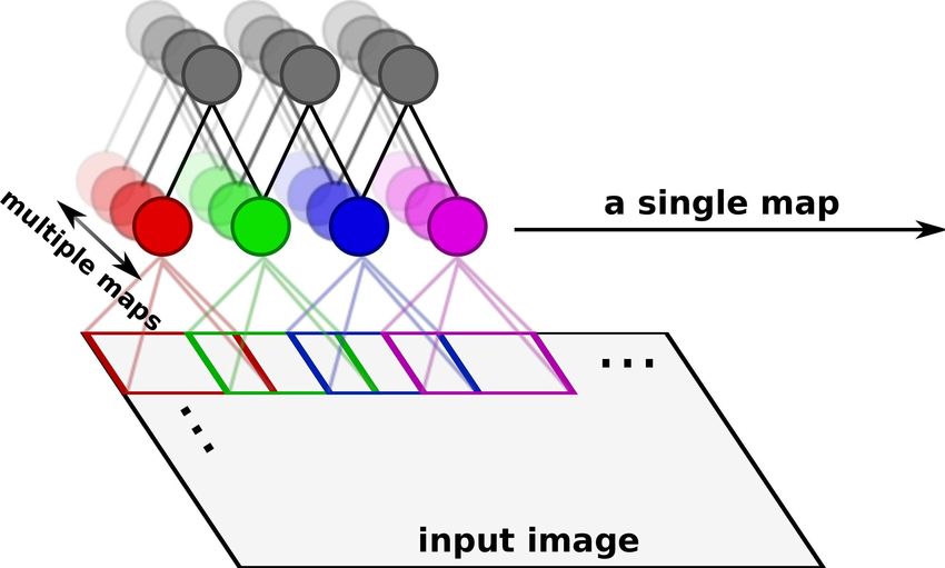
5than having each hidden unit connect to the entire input image, each unit is instead connected to a
small patch (see figure 2a for an illustration). This reduces the number of parameters in the model.
As a result, local receptive field neural networks are faster to optimize than their fully connected
counterparts. A major drawback of this approach, however, is the difficulty in enforcing orthogonal-
ity across partially overlapping patches. We show that swapping out locally enforced orthogonality
constraints with a global reconstruction cost solves this issue.
Specifically, we examine the local receptive field network proposed by Le et al. [12]. Their for-
mulation constrains each feature (a row of W ) to connect to a small region of the image (i.e., all
weights outside of the patch are set to zero). This modification allows learning ICA and TICA with
larger images, because W is now sparse. Unlike standard convolutional networks, these networks
may be extended to have fully unshared weights. This permits them to learn invariances other than
translational invariances, which are hardwired in convolutional networks.
The pre-training step for the TCNN (local receptive field TICA) [12] is performed by minimizing
the following cost function:
m X
X k q
minimize ǫ + Hj (W x(i) )2 , subject to W W T = I (9)
W
i=1 j=1
where H is the spatial pooling matrix and W is a learned weight matrix. The corresponding neural
network representation
p of this algorithm is one with two layers with weights W, H and nonlinearities
(.)2 and (.) respectively (see Figure 2a). In addition, W and H are set to be local. That is, each
row of W and H connects to a small region of the input data.
(a) Local receptive field neural net (b) Local orthogonalization (c) RICA global reconstruc-
tion cost
Figure 2: (a) Local receptive field neural network with fully untied weights. A single map consists
of local receptive fields that do not share a location (i.e., only different colored nodes). (b & c)
For illustration purposes we have brightened the area of each local receptive field within the input
image. (b) Hard orthonormalization [12] is applied at each location only (i.e., nodes of the same
color), which results in copied filters (for example, see the filters outlined in red; notice that the
location of the edge stays the same within the image even though the receptive field areas are differ-
ent). (c) Global reconstruction (this paper) is applied both within each location and across locations
(nodes of the same and different colors), which prevents copying of receptive fields.
Enforcing the hard orthonormality constraint on the entire sparse W matrix is challenging because it
is typically overcomplete for TCNNs. As a result, Le et al. [12] performed local orthonormalization
instead. That is, only the features (rows of W ) that share a location (e.g., only the red nodes in figure
2) were orthonormalized using symmetric orthogonalization.
However, visualizing the filters learned by a TCNN with local orthonormalization, shows that many
adjacent receptive fields end up learning the same (copied) filters due to the lack of an orthonormality
constraint between them. For instance, the green nodes in Figure 2 may end up being copies of the
red nodes (see the copied receptive fields in Figure 2b).
In order to prevent copied features, we replace the local orthonormalization constraint with a global
reconstruction cost (i.e., computing the reconstruction cost kW T W x(i) − x(i) k22 for the entire over-
complete sparse W matrix). Figure 2c shows the resulting filters. Figure 3 shows that the recon-
struction penalty produces a better distribution of edge detector locations within the image patch
(this also holds true for frequencies and orientations).
61 1
0.8 0.8
Vertical Location
Vertical Location
0.6 0.6
0.4 0.4
0.2 0.2
0 0
0 0.2 0.4 0.6 0.8 1 0 0.2 0.4 0.6 0.8 1
Horizontal Location Horizontal Location
Figure 3: Location of each edge detector within the image patch. Symbols of the same color/shape
correspond to a single map. Left: local orthonormalization constraint. Right: global reconstruction
penalty. The reconstruction penalty prevents copied filters, producing a more uniform distribution
of edge detectors.
6 Experiments
The following experiments compare the speed gains of RICA over standard overcomplete ICA. We
then use RICA to learn a large filter bank, and show that it works well for classification on the
STL-10 dataset.
6.1 Speed improvements for overcomplete ICA
In this experiment, we examine the speed performance of RICA and overcomplete ICA with score
matching [26]. We trained overcomplete ICA on 20000 gray-scale image patches, each patch of size
16x16. We learn representations that are 2x, 4x and 6x overcomplete. We terminate both algorithms
when changes in the parameter vector drop below 10−6 . We use the score matching implementation
provided in [16]. We report the time required to learn these representations in Table 2. The results
show that our method is much faster than the competing method. In particular, learning features that
are 6x overcomplete takes 1 hour using our method, whereas [26] requires 2 days.
Table 2: Speed improvements of our method over score matching [26].
2x overcomplete 4x overcomplete 6x overcomplete
Score matching ICA 33000 seconds 65000 seconds 180000 seconds
RICA 1000 seconds 1600 seconds 3700 seconds
Speed up 33x 40x 48x
Figure 4 shows the peak frequencies and orientations for 4x overcomplete bases learned using our
method. The learned bases do not degenerate, and they cover a broad range of frequencies and
orientations (cf. Figure 3 in [27]). This ability to learn a diverse set of features allows our algorithm
to perform well on various discriminative tasks.
Figure 4: Scatter plot of peak frequencies and orientations of Gabor functions fitted to the filters
learned by RICA on whitened images. Our model yields a diverse set of filters that covers the
spatial frequency space evenly.
6.2 Overcomplete ICA on STL-10 dataset
In this section, we evaluate the overcomplete features learned by our model. The experiments are
carried out on the STL-10 dataset [6] where overcomplete representations have been shown to work
well. The STL-10 dataset contains 96x96 pixel color images taken from 10 classes. For each
7class 500 training images and 800 test images are provided. In addition, 100,000 unlabeled images
are included for unsupervised learning. We use RICA to learn overcomplete features on 100,000
randomly sampled color patches from the unlabeled images in the STL-10 dataset. We then apply
RICA to extract features from images in the same manner described in [6].
Using the same number of features (1600) employed by Coates et al. [6] on 96x96 images and 10x10
receptive fields, our soft reconstruction ICA achieves 52.9% on the test set. This result is slightly
better than (but within the error bars) of the best published result, 51.5%, obtained by K-means [6].
50
51.5
Cross−Validation Accuracy (%)
45
40 soft ica
ica
Coates et al.
35 whitened
raw
30
25
0 200 400 600 800 1000 1200 1400 1600
Number of Features
Figure 5: Classification accuracy on the STL-10 dataset as a function of the number of bases learned
(for a patch size of 8x8 pixels). The best result shown uses bases that are 8x overcomplete.
Finally, we compare classification accuracy as a function of the number of bases. Figure 5 shows
the results for ICA and RICA. Notice that the reconstruction cost in RICA allows us to learn over-
complete representations that outperform the complete representation obtained by the regular ICA.
6.3 Reconstruction Independent Subspace Analysis for action recognition
Recently we presented a system [13] for learning features from unlabelled data that can lead to
state-of-the-art performance on many challenging datasets such as Hollywood2 [15], KTH [28]
and YouTube [29]. This system makes use of a two-layered Independent Subspace Analysis (ISA)
network [16]. Like ICA, ISA also uses orthogonalization for degeneracy control.4
In this section we compare the effects of reconstruction versus orthogonality on classification per-
formance using ISA. In our experiments we swap out the orthonormality constraint employed by
ISA with a reconstruction penalty. Apart from this change, the entire pipeline and parameters are
identical to the system described in [13].
We observe that the reconstruction penalty tends to works better than orthogonality constraints. In
particular, on the Hollywood2 dataset ISA achieves a mean AP of 54.6% when the reconstruction
penalty is used. The performance of ISA drops to 53.3% when orthogonality constraints are used.
Both results are state-of-the art resuls on this dataset [30]. We attribute the improvement in perfor-
mance to the fact that features in invariant subspaces of ISA need not be strictly orthogonal.
7 Discussion
In this paper, we presented a novel soft reconstruction approach that enables the learning of over-
complete representations in ICA and TICA. We have also presented mathematical proofs that con-
nect ICA with autoencoders and sparse coding. We showed that our algorithm works well even
without whitening; and that the reconstruction cost allows us to fix replicated filters in tiled convo-
lutional neural networks. Our experiments show that RICA is fast and works well in practice. In
particular, we found our method to be 30-50x faster than overcomplete ICA with score matching.
Furthermore, our overcomplete features achieve state-of-the-art performance on the STL-10 and
Hollywood2 datasets.
4
Note that in ISA the square nonlinearity is used in the first layer, and squareroot is used in in second
layer [13].
8References
[1] M.A. Ranzato, C. Poultney, S. Chopra, and Y. LeCun. Efficient learning of sparse representations with an
energy-based model. In NIPS, 2006.
[2] R. Raina, A. Battle, H. Lee, B. Packer, and A.Y. Ng. Self-taught learning: Transfer learning from unla-
belled data. In ICML, 2007.
[3] M. Ranzato, F. J. Huang, Y. Boureau, and Y. LeCun. Unsupervised learning of invariant feature hierarchies
with applications to object recognition. In CVPR, 2007.
[4] J. Yang, K. Yu, Y. Gong, and T. Huang. Linear spatial pyramid matching using sparse coding for image
classification. In CVPR, 2009.
[5] J. Yang, K. Yu, and T. Huang. Efficient highly over-complete sparse coding using a mixture model. In
ECCV, 2010.
[6] A. Coates, H. Lee, and A. Y. Ng. An analysis of single-layer networks in unsupervised feature learning.
In AISTATS 14, 2011.
[7] K. Yu, Y. Lin, and J. Lafferty. Learning image representations from pixel level via hierarchical sparse
coding. In CVPR, 2011.
[8] Y. Bengio, P. Lamblin, D. Popovici, and H. Larochelle. Greedy layerwise training of deep networks. In
NIPS, 2007.
[9] G. E. Hinton, S. Osindero, and Y. W. Teh. A fast learning algorithm for deep belief nets. Neural Compu-
tation, 2006.
[10] B. Olshausen and D. Field. Emergence of simple-cell receptive field properties by learning a sparse code
for natural images. Nature, 1996.
[11] A. Hyvärinen, J. Karhunen, and E. Oja. Independent Component Analysis. Wiley Interscience, 2001.
[12] Q. V. Le, J. Ngiam, Z. Chen, D. Chia, P. W. Koh, and A. Y. Ng. Tiled convolutional neural networks. In
NIPS, 2010.
[13] Q. V. Le, W. Zou, S. Y. Yeung, and A. Y. Ng. Learning hierarchical spatio-temporal features for action
recognition with independent subspace analysis. In CVPR, 2011.
[14] Q. V. Le, J. Ngiam, A. Coates, A. Lahiri, B. Prochnow, and A. Y. Ng. On optimization methods for deep
learning. In ICML, 2011.
[15] M. Marzalek, I. Laptev, and C. Schmid. Actions in context. In CVPR, 2009.
[16] A. Hyvärinen, J. Hurri, and P. O. Hoyer. Natural Image Statistics. Springer, 2009.
[17] B. Olshausen and D. Field. Sparse coding with an overcomplete basis set: A strategy employed by v1.
Vision Research, 1997.
[18] M. S. Lewicki and T. J. Sejnowski. Learning overcomplete representations. Neural Computation, 2000.
[19] L. Ma and L. Zhang. Overcomplete topographic independent component analysis. Elsevier, 2008.
[20] M. Schmidt. minFunc, 2005.
[21] P. Vincent, H. Larochelle, Y. Bengio, and P. A. Manzagol. Extracting and composing robust features with
denoising autoencoders. In ICML, 2008.
[22] H. Lee, C. Ekanadham, and A. Y. Ng. Sparse deep belief net model for visual area V2. In NIPS, 2008.
[23] H. Larochelle, Y. Bengio, J. Louradour, and P. Lamblin. Exploring strategies for training deep neural
networks. JMLR, 2009.
[24] G. Hinton. A practical guide to training restricted boltzmann machines. Technical report, U. of Toronto,
2010.
[25] P. Vincent. A connection between score matching and denoising autoencoders. Neural Computation,
2010.
[26] A. Hyvärinen. Estimation of non-normalized statistical models using score matching. JMLR, 2005.
[27] Y. Karklin and M.S. Lewicki. Is early vision optimized for extracting higher-order dependencies? In
NIPS, 2006.
[28] C. Schuldt, I. Laptev, and B. Caputo. Recognizing human actions: A local SVM approach. In ICPR,
2004.
[29] J. Liu, J. Luo, and M. Shah. Recognizing realistic actions from videos “in the Wild”. In CVPR, 2009.
[30] Heng Wang, Muhammad Muneeb Ullah, Alexander Klaser, Ivan Laptev, and Cordelia Schmid. Evaluation
of local spatio-temporal features for action recognition. In BMVC, 2010.
9You can also read