PRE-INTERPOLATION LOSS BEHAVIOUR IN NEURAL NETWORKS - CAIR
←
→
Page content transcription
If your browser does not render page correctly, please read the page content below
P RE - INTERPOLATION L OSS B EHAVIOUR IN N EURAL
                                                                       N ETWORKS

                                                                                               A P REPRINT

                                                                 Arthur E.W. Venter, Marthinus W. Theunissen, Marelie H. Davel
                                                   Multilingual Speech Technologies, North-West University, South Africa; and CAIR, South Africa.
arXiv:2103.07986v1 [cs.LG] 14 Mar 2021

                                                    aew.venter@gmail.com, tiantheunissen@gmail.com, marelie.davel@nwu.ac.za

                                                                                              March 16, 2021

                                                                                               A BSTRACT
                                                  When training neural networks as classifiers, it is common to observe an increase in average test
                                                  loss while still maintaining or improving the overall classification accuracy on the same dataset.
                                                  In spite of the ubiquity of this phenomenon, it has not been well studied and is often dismissively
                                                  attributed to an increase in borderline correct classifications. We present an empirical investigation
                                                  that shows how this phenomenon is actually a result of the differential manner by which test samples
                                                  are processed. In essence: test loss does not increase overall, but only for a small minority of samples.
                                                  Large representational capacities allow losses to decrease for the vast majority of test samples at the
                                                  cost of extreme increases for others. This effect seems to be mainly caused by increased parameter
                                                  values relating to the correctly processed sample features. Our findings contribute to the practical
                                                  understanding of a common behaviour of deep neural networks. We also discuss the implications of
                                                  this work for network optimisation and generalisation.

                                         Keywords Overfitting · generalisation · Deep learning

                                         1   Introduction
                                         According to the principal of empirical risk minimisation, it is possible to optimise the performance on machine learning
                                         tasks (e.g. classification or regression) by reducing the empirical risk on a surrogate loss function as measured on a
                                         training dataset [1]. The success of this depends on several assumptions regarding the sampling methods used to obtain
                                         the training data and the consistency of the risk estimators [2]. Assuming such criteria are met, we expect the training
                                         loss to decrease throughout training and that the loss on samples not belonging to the training samples (henceforth
                                         referred to as validation or evaluation loss) will initially decrease but eventually increase as a result of overfitting on
                                         spurious features in the training set.
                                         Actual performance is usually not directly measured with the loss function but rather with a secondary measurement,
                                         such as classification accuracy in a classification task. It is implicitly expected that the classification accuracy will be
                                         inversely proportional to the average loss value. However, in practice we often observe that the validation loss increases
                                         while the validation accuracy is stable or still improving, as illustrated by the example in Fig. 1.
                                         The cause of this behaviour can easily be thought to be shallow local optima or borderline cases of correct classification.
                                         While this explanation is consistent with classical ideas of overfitting, it does not fully explain observed behaviour.
                                         Specifically, if this is the extent of the phenomenon, there is no reason for improvement in validation accuracy if a local
                                         optimum is found, and an obvious quantitative limit to the amount that the validation loss can increase.
                                         By investigating the distribution of per-sample validation loss values and not just a point estimation (typically averaged
                                         over all samples) we show that the increase in average validation loss can be attributed to a minority of validation
                                             The final authenticated publication is available online at https://doi.org/10.1007/978-3-030-66151-9_19
A PREPRINT - M ARCH 16, 2021
Figure 1: Learning curves of an example 1 × 1 000 MLP trained on 5 000 FMNIST samples using SGD with a
mini-batch size of 64. The network clearly shows an increasing validation loss with a slightly increasing validation
accuracy.
samples. This means that the discrepancy between the validation loss and accuracy is due to a form of overfitting that
only affects the predictions of some validation samples, thereby allowing the model to still generalise well to most of
the validation set.
The following is a summary of the main contributions of this paper:
• We present empirical evidence of a characteristic of empirical risk minimisation in MLPs performing classifica-
tion tasks, that sheds light on an apparently paradoxical relationship between validation loss and classification
accuracy.
• We explain how this phenomenon is largely a result of quantitative increases in related parameter values and
the limits of using a point estimator to measure overfitting.
• We discuss the practical and theoretical implications of this phenomenon with regards to generalisation in
related machine learning models.
In the following section we discuss related work. In Section 3 we explain our experimental setup and methodology.
Section 4 presents our empirical results and their interpretation. The final section discusses and summarizes our findings
with a focus on their implications for generalisation.
2 Background
Much work has been done to characterize how a neural network’s performance changes over training iterations
[3, 4, 5, 6]. Such work has lead to some powerful machine learning techniques, including drop-out [7] and batch
normalisation [8]. While both theoretically principled and practically useful generalisation bounds remain out of reach,
many heuristics have been found that appear to indicate whether a trained neural network will generalise well. These
heuristics have varying degrees of complexity, generality, and popularity, and include: small weight norms, flatness of
loss landscapes [9], heavy-tailed weight matrices [10], and large margin distributions [11]. All of these proposed metrics
have empirical evidence to support their claims of contributing to the generalisation ability of a network, however, none
of them have been proven to be a sufficient condition to ensure generalisation in general circumstances.
A popular experimental framework used to investigate generalisation in deep learning is to explore the optimisation
process of so-called “toy problems". Such experiments are typically characterized by varying different design choices
2A PREPRINT - M ARCH 16, 2021
or training conditions, in an often simplified machine learning model, and then interpreting the performance of resulting
models on test data [12, 13]. The performance can be investigated post-training but it is often informative to observe
how the generalisation changes during training.
A good example of why it is important to consider performance during training is the double descent phenomenon
[14, 15]. This phenomenon has enjoyed much attention recently [?, 16, 17], due to its apparent bridging of classical and
modern regimes of representational complexity. In its most basic form it is characterized by poor generalisation within
a “critically parameterized" regime of representational capacities near the minimum that is necessary to interpolate the
entire training set. Slightly smaller or larger models produce improved generalisation. However, if early stopping is
used the phenomenon has been found to be almost non-existent [15].
Having an accurate estimate of test loss and how it changes during training is clearly beneficial in investigating
generalisation. In the current work we show that averaging over all test samples can result in a misrepresentation of
generalisation ability and that this can account for the sometimes paradoxical relationship between test accuracy and
test loss.
3 Approach
We use a simple experimental setup to explore the validation loss behaviour of various fully-connected feedforward
networks. All models use a multilayer perceptron (MLP) architecture where hidden layers have an equal number of
ReLU-activated nodes. This architecture, while simple, still uses the fundamental principles common to many deep
learning models, that is, a set of hidden layers optimised by gradient descent, using backpropagation to calculate the
gradient of a given loss function with regard to the parameters being optimised.
We first determine whether the studied phenomenon (both validation accuracy and loss displaying an increase during
training) occurs in general circumstances, and then select a few models where this phenomenon is clearly visible. We
then probe these models to better understand the mechanism causing this effect.
The experiments are performed on the well-known MNIST [18] and FMNIST [19] classification datasets. These
datasets consist of 60 000 training samples and 10 000 test samples of 28 × 28 grayscale images with an associated label
∈ [0, 9]. FMNIST can be regarded as a slightly more complex drop-in replacement for MNIST. Recently these datasets
have become less useful as benchmarks, but they are still popular resources for investigating theoretical principles of
DNNs.
All models are optimised to reduce a cross-entropy loss function measured on mini-batches of training samples.
Techniques that could have a regularizing effect on the optimisation process (such as batch normalisation, drop-out,
early-stopping or weight decay) were omitted as far as possible. Networks are trained till convergence, with the exact
stopping criteria different for the separate experiments, as described per set of results.
A selection of hyperparameters were investigated to ensure a variety of validation loss behaviours during training. These
hyperparameters are:
• Training and validation set sizes;
• The number of hidden layers;
• The number of nodes in each hidden layer;
• Mini-batch sizes;
• Datasets (MNIST or FMNIST); and
• optimisers (Adam or SGD).
Parameter settings differed per experiment, as detailed below. Take note that the validation sets are held out from the
train set, so a larger train set will result in a smaller validation set and vice versa.
4 Results
Our initial experiments show that the average validation loss can indeed increase with a stable or increasing validation
accuracy for a wide variety of hyperparameters (Section 4.1). Based on this result, we select a few models where the
phenomenon is clearly visible, and investigate the per-sample loss distributions throughout training, as well as weight
distributions, to probe the reason for this behaviour (Sections 4.2 and 4.3).
3A PREPRINT - M ARCH 16, 2021
4.1 Increasing Risk During Training
We begin our investigation by training 95 two-layer MLPs, varying the width of the hidden layer and the optimisation
algorithm over multiple random initialisations. Networks are trained on 5 000 MNIST training samples using a
mini-batch size of 64. All models were trained until interpolation (training accuracy of 100%), which occurred at
around 3 000 epochs for the smaller models. Out of the 95 models trained, 57 (3 initialisations of 19 widths) were
optimised with Adam and the remaining 38 (2 initialisations of 19 widths) with SGD.
The results are presented in the scatter plots in Fig. 2. The measurement for the horizontal axis is made at the epoch
where the model achieved the lowest validation loss. The measurement for the vertical axis is made at the epoch where
the model first interpolated the entire training set. Using the linear curve as reference, all models falling above the line
increased the relevant metric after the point of minimum validation loss. The models marked by a triangle saw increases
in both validation loss and accuracy.
Notice that the models with limited representational capacity, in this case referring to the number of nodes in the hidden
layer, had increasing validation loss and decreasing validation accuracy as one would expect. This is in contrast with
the larger models that tend to display an increase in both validation accuracy and loss even before interpolation. An
additional observation we can make is that a higher minimum validation loss seems to be indicative of very large
increases in validation loss later in training.
We repeated this experiment in a more general setting to produce the results presented in Fig. 3. These models have
hyperparameters that vary beyond just the hidden layer width and optimiser. Specifically:
• The data is either MNIST or FMNIST with a train set size as defined in the legend;
• The number of hidden layers is either 1, 3, or 10;
• The number of nodes in each hidden layer is either 100 or 1000;
• Mini-batch sizes are either 16, 64 or 256; and
• The optimisers are again either Adam or SGD.
Figure 2: Final validation loss (left) and validation accuracy (right) vs the same metric at the epoch with minimum
validation loss. 95 MLPs are trained on 5 000 MNIST samples with the number of nodes in the hidden layer ranging
from only 7 (red) to 2 000 (blue). Models marked with a triangle had increasing validation loss and accuracy between
the epoch of minimum validation loss and the epoch of first interpolation.
These networks are trained for 150 epochs. In order to ensure that each model’s performance is good enough to be
considered typical for these architectures and datasets, we use optimised learning rates. The learning rate for each set of
hyperparameters is chosen by a grid search over a wide range of values. The selection is made in accordance with the
4A PREPRINT - M ARCH 16, 2021
Figure 3: Final validation loss (left) and validation accuracy (right) vs the same metric at the epoch with minimum
validation loss. 80 MLPs are trained with varying hyperparameters; colours refer to different training sets. Models
marked with a triangle had increasing validation loss and accuracy between the epoch of minimum validation loss and
the epoch of first interpolation.
best validation error achieved by the end of training. In some cases this resulted in final training accuracies slightly
below 100%. In these cases we selected the “final" epoch at the epoch where maximum training accuracy was achieved.
As expected, the models trained on MNIST or on larger training sets had lower validation losses and higher validation
accuracies in general. However, we also note that models trained on FMNIST tend to have much higher increases in
validation loss while the validation accuracy is still improving when compared to models trained on MNIST. In the next
section we investigate how the loss distributions change for selected models from this section.
4.2 Loss Distributions
In order to take a closer look at how both loss and accuracy can increase during training, we present a case study of four
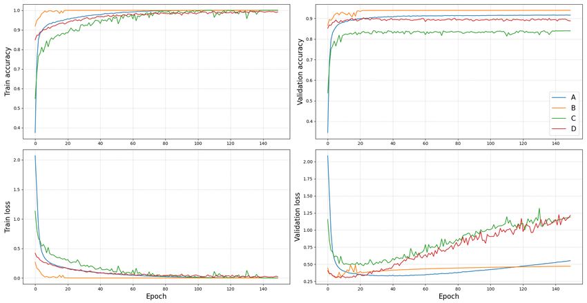
selected models from the previous section. They are defined below.
• A: 3x100 model trained on 5 000 MNIST samples using Adam and a mini-batch size of 64.
• B: 3x100 model trained on 5 000 MNIST samples using SGD and a mini-batch size of 64.
• C: 3x100 model trained on 5 000 FMNIST samples using SGD and a mini-batch size of 64.
• D: 3x100 model trained on 55 000 FMNIST samples using Adam and a mini-batch size of 16.
The learning curves for these models are presented in Fig. 4. Notice that for all four models a minimum validation loss
is achieved early on. Beyond this point the validation loss increases while the corresponding accuracy is either stable or
improving slightly.
The validation loss curve, as seen in Fig. 4, is often used as an estimate of the level of overfitting that is occurring as the
model is optimised on the training set. However, by averaging over the entire validation set we are producing a point
estimate that implicitly assumes that the loss of all validation samples are close to the mean value. This assumption is
reasonable with regards to the training set because most loss functions (e.g. cross entropy) work with the principle of
maximum likelihood estimation [2, 1]. This means that by minimizing the dissimilarity between the entire distribution
of the training data and the model the estimate of loss is all but guaranteed to be indicative of performance on the entire
training set.
There is no such guarantee with regards to any set other than the training set. This makes the average loss value a poor
estimate of performance on the validation set. The results presented in Fig. 5 motivate this point for model A. See
5A PREPRINT - M ARCH 16, 2021
Figure 4: Learning curves for four selected models (A-D, see text) showing increasing validation loss, despite an
increasing or stable validation accuracy.
Appendix. A for the same results for models B, C, and D. The plots show heatmaps of loss distributions for the four
selected models at several training iterations for three datasets (training, validation and evaluation). The validation set
is the held-out set that is used to estimate performance during training and model selection, and the evaluation set is
the set that is used post-training to ensure no indirect optimisation is performed on the test data. The iterations refer
to parameter updates, not epochs. We show the distributions at log-sampled iterations because many changes occur
early on (even before the end of the first epoch) and few occur towards the end of training. A final note with regards to
these heatmaps is that the colours, which define the number of samples that have the corresponding loss value, are also
log-scaled. This visually highlights the occurrence of samples with extreme loss values.
The loss distributions in Fig. 5 show that while the loss value for a vast majority (indicated by the red and orange
colours) of samples reduces with training iterations there is a small minority of samples for which the loss values
increase. For the training set, this increase is relatively low and eventually reduces as the entire set is interpolated. For
the validation and evaluation sets the loss values of these “outliers" seem to only increase. This is why it is possible for
the average validation loss to increase while the classification accuracy remains stable or improves.
Fig. 6 shows the weight distributions for the same model in the same format as Fig. 5. See Appendix. A for models B,
C, and D. It can be observed that there is a clear increase in the magnitude of some weights (their absolute weight
values) at the same iterations where we observe a corresponding increase in validation and evaluation loss values in
Fig. 5. This appears to occur even more after most of the training sample losses have been minimized. This is consistent
with the notion of limiting weight norms to improve generalisation and it suggests that the reason for the increase in
validation losses is because particular weights are being increased to fit idiosyncratic training samples.
While these heatmaps show that there are outlier per-sample loss values in the validation set, they do not guarantee that
these extreme loss values are due to specific samples. It is possible that the extreme values are measured on completely
different samples at every measured iteration, in which case there is nothing extreme about them and the phenomenon
has something to do with the optimisation process and not training and validation distributions. We address this question
in the next section.
4.3 Validation Set Outliers
In this section we investigate whether the validation set samples with extreme loss values are individual samples that
are consistently modeled poorly, or whether these outliers change from iteration to iteration due to the stochastic nature
of the optimisation process. Towards this end, we analyze the number of epochs for which a sample can be regarded as
an outlier and compare it with its final loss value.
6A PREPRINT - M ARCH 16, 2021
Figure 5: Change in loss distributions during training for model A (5k MNIST, Adam, mini-batch size of 64). The three
heatmaps refer to the train (top), validation (center), and evaluation (bottom) loss distributions.
Figure 6: Change in weight distributions during training for model A (MNIST, Adam, mini-batch size of 64). Each
heatmap refers to a layer in the network, including the output layer, from top to bottom.
7A PREPRINT - M ARCH 16, 2021
We classify a sample as an outlier when its loss value is above the upper Tukey fence, that is, larger than Q3 + 1.5 ×
(Q3 − Q1 ), where Q1 and Q3 are the first and third quartile of all loss values in the validation set, respectively [20].
This indicator is simple and adequate to illustrate whether some specific samples consistently have much larger loss
values than the majority.
In Fig. 7 we show that the validation samples with extreme loss values at the end of training are usually classified as
outliers for most of the training process. This means that the extreme validation loss values are due to specific samples
that are not well modeled. In addition to this, it is worth observing that a large majority of validation samples are never
classified as an outlier and these samples always have small loss values at the end of training.
(a) A: Fitting 5k MNIST; Adam (b) B: Fitting 5k MNIST; SGD
(c) C: Fitting 5k FMNIST; SGD (d) D: Fitting 55k FMNIST; Adam
Figure 7: Outliers in the validation set. The blue datapoints show the number of epochs for which each sample is
considered an outlier. The red datapoints show the loss value of each sample at the end of training. Samples are ordered
in ascending order of epoch counts.
5 Discussion
We have shown that validation classification accuracy can increase while the corresponding average loss value also
increases. Empirically, we have noted that this phenomenon is most influenced by the interplay between the training
dataset and model capacity. Specifically, it occurs more for larger models, smaller training datasets, and more difficult
datasets (FMNIST in our investigation). We can, however, combine the first and second factors because capacity is
directly related to the size and complexity of the training set.
By taking a closer look at per-sample loss distributions and weight distributions we have noted that the phenomenon is
largely due to specific samples in the validation set that have extremely large loss values and obtain progressively larger
loss values as training continues. These loss values then become large enough to distort the average loss value in such
a way that it appears that the model is overfitting the training set, when most of the validation set sample losses are
still being minimized. From a theoretical viewpoint this is unsurprising because the average validation loss is only a
good measure of risk with regards to the train set, where it is directly being minimized by the principle of maximum
likelihood estimation. From a practical viewpoint it appears that increased weight values are sacrificing the generality
of the distributed representation used by DNNs in order to minimize training loss as much as possible.
8A PREPRINT - M ARCH 16, 2021
Practically, these findings serve as a clear cautionary tale for (1) assuming an inverse correlation between loss and
accuracy, and for (2) measuring overfitting with point estimators such as average validation loss. Rather, we show that
loss distribution heatmaps (Fig. 5) provide additional, useful information.
The findings also highlight a more general aspect of generalisation and deep learning: DNNs optimise parameters with
regards to training data in a heterogeneous manner. With sufficient parametric flexibility, these types of models can fit
generalisable features and memorize non-generalisable features concurrently during training. Formally defining how
this is achieved, and subsequently, how generalisation should be characterized in this context, remains an open problem.
6 Conclusion
By means of a small but focused empirical investigation we have contributed the following findings, in the context of
using fully-connected feedforward networks as classifiers:
• If the representational capacity is large enough, validation classification accuracy and loss can both increase
simultaneously during training.
• Under common conditions, average validation loss is a poor estimate of generality because validation samples
are not guaranteed to obtain loss values near the mean value.
• We show that sample-specific heatmaps provide a far more nuanced view of the training process, and can be a
useful tool during model optimisation.
• We propose that investigations of generalisation should consider the fact that DNN optimisation is distributed
and heterogeneous, which is why simple measures of overfitting can be misleading.
These findings imply that a validation loss that starts increasing prior to interpolation of the training set is not necessarily
an implication of overfitting; and also that it is dangerous to assume a negative correlation between validation accuracy
and loss (which is often done when selecting hyperparameters).
While this study aimed to answer a very specific question, we hope it will contribute to the general discourse on factors
that influence the optimisation process and generalisation ability of neural networks.
9A PREPRINT - M ARCH 16, 2021
A Appendix
We include the results when models B, C and D are analyzed, using the same process as described in Section 4.2.
(a) B: Fitting 5k MNIST; SGD (b) B: Fitting 5k MNIST; SGD
(c) C: Fitting 5k FMNIST; SGD (d) C: Fitting 5k FMNIST; SGD
(e) D: Fitting 55k FMNIST; Adam (f) D: Fitting 55k FMNIST; Adam
Figure 8: Change in loss (left) and weight (right) distributions, for models B, C, and D, during training. See Fig. 5 and
6 for plot ordering.
References
[1] Ian Goodfellow, Yoshua Bengio, and Aaron Courville. Deep Learning. MIT Press, 2016. http://www.
deeplearningbook.org.
[2] Kevin P. Murphy. Machine Learning: A Probabilistic Perspective. The MIT Press, 2012.
[3] D. R. Wilson and T. Martinez. The general inefficiency of batch training for gradient descent learning. Neural
networks : the official journal of the International Neural Network Society, 16 10:1429–51, 2003.
10A PREPRINT - M ARCH 16, 2021
[4] Behnam Neyshabur, Ryota Tomioka, and Nathan Srebro. In search of the real inductive bias: On the role of
implicit regularization in deep learning. CoRR, abs/1412.6614, 2015.
[5] Moritz Hardt, Ben Recht, and Yoram Singer. Train faster, generalize better: Stability of stochastic gradient descent.
In International Conference on Machine Learning, pages 1225–1234. PMLR, 2016.
[6] Elad Hoffer, Itay Hubara, and Daniel Soudry. Train longer, generalize better: closing the generalization gap in
large batch training of neural networks. In Advances in Neural Information Processing Systems, pages 1731–1741,
2017.
[7] Geoffrey E. Hinton, Nitish Srivastava, Alex Krizhevsky, Ilya Sutskever, and Ruslan Salakhutdinov. Improving
neural networks by preventing co-adaptation of feature detectors. CoRR, abs/1207.0580, 2012.
[8] Sergey Ioffe and Christian Szegedy. Batch normalization: Accelerating deep network training by reducing internal
covariate shift. In Proceedings of the 32nd International Conference on Machine Learning, 2015, Lille, France,
6-11 July 2015, volume 37 of JMLR Workshop and Conference Proceedings, pages 448–456. JMLR.org, 2015.
[9] S. Hochreiter and J. Schmidhuber. Flat minima. Neural Computation, 9:1–42, 1997.
[10] C. Martin and M. Mahoney. Implicit self-regularization in deep neural networks: Evidence from random matrix
theory and implications for learning. ArXiv, abs/1810.01075, 2018.
[11] Jure Sokolic, Raja Giryes, G. Sapiro, and M. Rodrigues. Robust large margin deep neural networks. IEEE
Transactions on Signal Processing, 65:4265–4280, 2017.
[12] Roman Novak, Yasaman Bahri, Daniel A. Abolafia, Jeffrey Pennington, and Jascha Sohl-Dickstein. Sensitivity and
generalization in neural networks: an empirical study. In International Conference on Learning Representations,
2018.
[13] Ian J. Goodfellow and Oriol Vinyals. Qualitatively characterizing neural network optimization problems. CoRR,
abs/1412.6544, 2015.
[14] M. Belkin, Daniel Hsu, Siyuan Ma, and Soumik Mandal. Reconciling modern machine-learning practice and the
classical bias–variance trade-off. Proceedings of the National Academy of Sciences, 116:15849 – 15854, 2019.
[15] Preetum Nakkiran, Gal Kaplun, Yamini Bansal, Tristan Yang, Boaz Barak, and Ilya Sutskever. Deep double
descent: Where bigger models and more data hurt. In International Conference on Learning Representations,
2020.
[16] Stéphane d’Ascoli, Maria Refinetti, G. Biroli, and F. Krzakala. Double trouble in double descent: Bias and
variance(s) in the lazy regime. In Thirty-seventh International Conference on Machine Learning, pages 2676–2686,
2020.
[17] Preetum Nakkiran, Prayaag Venkat, Sham M. Kakade, and Tengyu Ma. Optimal regularization can mitigate
double descent. ArXiv, abs/2003.01897, 2020.
[18] Yann Lecun, Leon Bottou, Y. Bengio, and Patrick Haffner. Gradient-based learning applied to document
recognition. Proceedings of the IEEE, 86:2278 – 2324, 12 1998.
[19] Han Xiao, Kashif Rasul, and Roland Vollgraf. Fashion-MNIST: a novel image dataset for benchmarking machine
learning algorithms. CoRR, abs/1708.07747, 2017.
[20] J.L. Devore and Nicholas R. Farnum. Applied Statistics for Engineers and Scientists. Thomson Brooks/Cole,
2005.
11You can also read