IMAGE PROCESSING I Getting Started - Michael Habeck November 4, 2020

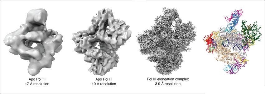
IMAGE PROCESSING I
Getting Started

Michael Habeck
November 4, 2020
michael.habeck@uni-jena.de

Microscopic Image Analysis
University Hospital Jena

OVERVIEW

 ∙ Course organization
 ∙ Why do we need image processing?
 ∙ Levels of image processing
 ∙ Doing image processing with computer programs
 ∙ Python

 1

COURSE ORGANIZATION

 Lecturers

 ∙ Michael Habeck (Microscopic Image Analysis)
 ∙ Christoph Biskup (Biomolecular Photonics)
 ∙ Fengjiao Ma, Rainer Heintzmann (Institute of Physical Chemistry,
 Bio-Nanoimaging Group)

 Course organization

 ∙ weekly lecture (Wednesday 10:15 – 11:45)
 ∙ and exercise (Wednesday 13:00 - 14:30) via zoom
 ∙ visit the course page for material and links to exercise, zoom
 meeting, etc.

 2

https://www.uniklinikum-jena.de/medpho/en/Semester+
information/Winter+term+2020_2021/1st+semester/Module+F1_
1+_+Image+Processing+I.html

 3

medpho_student Ilikephotonics

 4

SOME USEFUL REFERENCES
 ∙ R. Chityala & S. Pudipeddi: Image Processing and Acquisition Using
 Python (CRC Press, 2020)
 ∙ T. Salditt, T. Aspelmeier & S. Aeffner: Biomedical Imaging (DeGryter,
 2017)
 ∙ B. Jähne: Digital Image Processing (Springer, 2005)
 ∙ D. Beazley & B. Jones: Python Cookbook: Recipes for Mastering
 Python 3 (O’Reilly, 2013)
 ∙ J. VanderPlas: A Whirlwind Tour of Python (O’Reilly, 2016)

 5

WHY DO WE NEED IMAGE PROCESSING?
 Image processing is cross-disciplinary and essential in many fields of
 science

 from: Nature 568, 284-285 (2019)

 6

WHY DO WE NEED IMAGE PROCESSING?

 Segmentation in medical imaging

 from: https://commons.wikimedia.org from: https://commons.wikimedia.org

 7

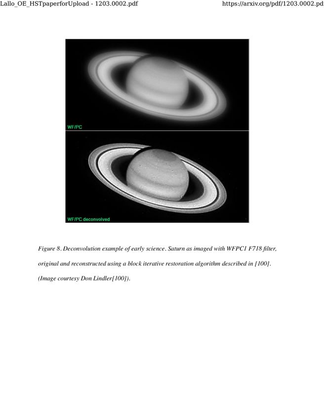
WHY DO WE NEED IMAGE PROCESSING?

 Sharpening images by deconvolution https://arxiv.org/pdf/1203.0002.pdf

 from: M. D. Lallo: Opt. Eng. (2012) 51 from: J.-B. Sibarita: Adv Biochem Engin/Biotechnol (2005) 95: 201– 243

 8

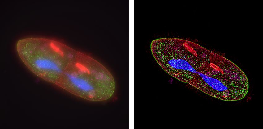
WHY DO WE NEED IMAGE PROCESSING?

 from: https://www.leica-microsystems.com/science-lab/introduction-to-widefield-microscopy

 9

SINGLE-PARTICLE ANALYSIS IN CRYO-EM

 Electron beam

 Ice layer

 Micrograph

 1

 10

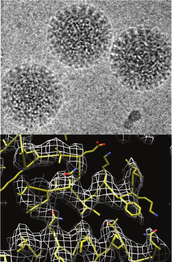
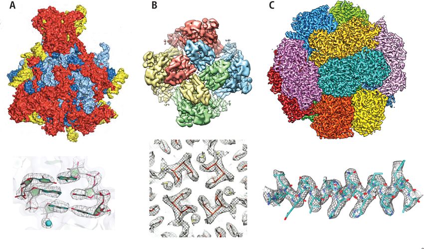
SINGLE-PARTICLE ANALYSIS IN CRYO-EM

 The resolution revolution: from ’blobology’ to near-atomic resolution

 from: J. Hanske, Y. Sadian & C. W. Müller: Curr. Opin. Struc. Biol. (2018) 52:8-15

 11

SINGLE-PARTICLE ANALYSIS IN CRYO-EM

 Motion correction

 from: D. Elmlund & H. Elmlund: Annu. Rev. Biochem. (2015) 84:499–517
 X. Bai, G. McMullan & S. H. W. Scheres: TIBS (2015) 40:49-57

 12

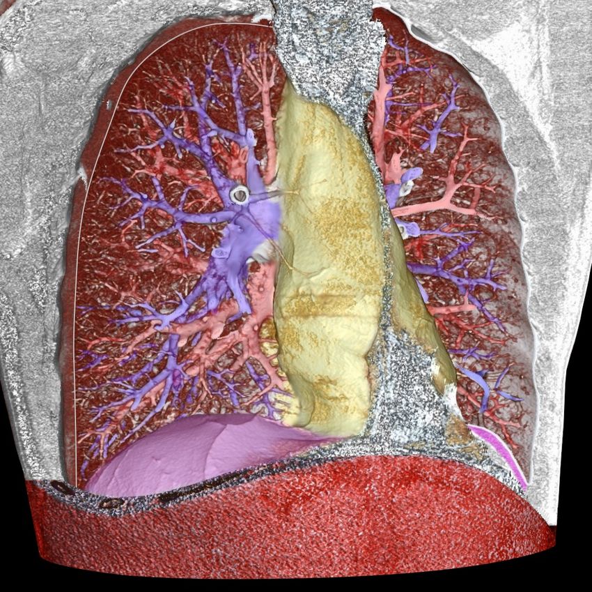
SINGLE-PARTICLE ANALYSIS IN CRYO-EM
 Particle Picking

 from: R. Hall & A. Patwardhan: J. Struct. Biol. (2004) 145:19-28

 13

SINGLE-PARTICLE ANALYSIS IN CRYO-EM
 Class averaging

 from: R. Hall & A. Patwardhan: J. Struct. Biol. (2004) 145:19-28

 14

SINGLE-PARTICLE ANALYSIS IN CRYO-EM
 Ab initio reconstruction

 from: P. Joubert & M. Habeck: Biophys. J. (2015) 108:1165-1175

 15

SINGLE-PARTICLE ANALYSIS IN CRYO-EM
 Structure refinement

 from: W. Kühlbrandt: Science (2014) 343:1443-1444

 16

LEVELS OF COMPUTERIZED IMAGE PROCESSING

 Low-level processes involve primitive operations such as
 ∙ preprocessing to reduce noise
 ∙ contrast enhancement
 ∙ image sharpening
 Input and output are typically images

 17

LEVELS OF COMPUTERIZED IMAGE PROCESSING

 Low-level processes involve primitive operations such as
 ∙ preprocessing to reduce noise
 ∙ contrast enhancement
 ∙ image sharpening
 Input and output are typically images
 Mid-level processes involve tasks such as
 ∙ segmentation
 ∙ classification of individual objects
 Attributes are extracted from images

 17

LEVELS OF COMPUTERIZED IMAGE PROCESSING

 Low-level processes involve primitive operations such as
 ∙ preprocessing to reduce noise
 ∙ contrast enhancement
 ∙ image sharpening
 Input and output are typically images
 Mid-level processes involve tasks such as
 ∙ segmentation
 ∙ classification of individual objects
 Attributes are extracted from images
 High-level processes involve operations such as
 ∙ image analysis
 ∙ cognitive functions associated with human vision

 17

SOME DEFINITIONS

 An image is a two-dimensional function ( , )
 where and are spatial coordinates
 32

 a
 b

 l

 m

 y
 n

 Figure 2.1: Representation of digital images by arr
 rectangular grid: a 2-D image, b 3-D image.

 is given in the common notation for matrices.
 notes the position of the row, the second, n, the
 (Fig. 2.1a). If the digital image contains M × N p
 by an M × N matrix, the index n runs from 0 to
 from 0 to M − 1. M gives the number of rows, N
 In accordance with the matrix notation, the ve
 from top to bottom and not vice versa as it is c
 from: B. Jähne: Digital Image Processing (Fig 2.1) horizontal axis (x axis) runs as usual from left t
 Each pixel represents not just a point in the im
 gular region, the elementary cell of the grid. Th
 the pixel must represent the average irradiance i
 in an appropriate way. Figure 2.2 shows one 18 an
 sented with a different number of pixels as indic

SOME DEFINITIONS

 An image is a two-dimensional function ( , )
 where and are spatial coordinates
 32

 ( , ) is the intensity or gray level of the image a

 at point ( , ) b

 l

 m

 y
 n

 Figure 2.1: Representation of digital images by arr
 rectangular grid: a 2-D image, b 3-D image.

 is given in the common notation for matrices.
 notes the position of the row, the second, n, the
 (Fig. 2.1a). If the digital image contains M × N p
 by an M × N matrix, the index n runs from 0 to
 from 0 to M − 1. M gives the number of rows, N
 In accordance with the matrix notation, the ve
 from top to bottom and not vice versa as it is c
 from: B. Jähne: Digital Image Processing (Fig 2.1) horizontal axis (x axis) runs as usual from left t
 Each pixel represents not just a point in the im
 gular region, the elementary cell of the grid. Th
 the pixel must represent the average irradiance i
 in an appropriate way. Figure 2.2 shows one 18 an
 sented with a different number of pixels as indic

SOME DEFINITIONS

 An image is a two-dimensional function ( , )
 where and are spatial coordinates
 32

 ( , ) is the intensity or gray level of the image a

 at point ( , ) b

 When all coordinates ( , ) and intensities ( , ) l

 are finite, discrete quantities, the image is a
 m

 digital image
 y
 n

 Figure 2.1: Representation of digital images by arr
 rectangular grid: a 2-D image, b 3-D image.

 is given in the common notation for matrices.
 notes the position of the row, the second, n, the
 (Fig. 2.1a). If the digital image contains M × N p
 by an M × N matrix, the index n runs from 0 to
 from 0 to M − 1. M gives the number of rows, N
 In accordance with the matrix notation, the ve
 from top to bottom and not vice versa as it is c
 from: B. Jähne: Digital Image Processing (Fig 2.1) horizontal axis (x axis) runs as usual from left t
 Each pixel represents not just a point in the im
 gular region, the elementary cell of the grid. Th
 the pixel must represent the average irradiance i
 in an appropriate way. Figure 2.2 shows one 18 an
 sented with a different number of pixels as indic

SOME DEFINITIONS

 An image is a two-dimensional function ( , )
 where and are spatial coordinates
 32

 ( , ) is the intensity or gray level of the image a

 at point ( , ) b

 When all coordinates ( , ) and intensities ( , ) l

 are finite, discrete quantities, the image is a
 m

 digital image
 A digital image is composed of a finite number of y
 n

 elements, each of which has a particular location Figure 2.1: Representation of digital images by arr
 rectangular grid: a 2-D image, b 3-D image.
 and value
 is given in the common notation for matrices.
 notes the position of the row, the second, n, the
 (Fig. 2.1a). If the digital image contains M × N p
 by an M × N matrix, the index n runs from 0 to
 from 0 to M − 1. M gives the number of rows, N
 In accordance with the matrix notation, the ve
 from top to bottom and not vice versa as it is c
 from: B. Jähne: Digital Image Processing (Fig 2.1) horizontal axis (x axis) runs as usual from left t
 Each pixel represents not just a point in the im
 gular region, the elementary cell of the grid. Th
 the pixel must represent the average irradiance i
 in an appropriate way. Figure 2.2 shows one 18 an
 sented with a different number of pixels as indic

SOME DEFINITIONS

 An image is a two-dimensional function ( , )
 where and are spatial coordinates
 32

 ( , ) is the intensity or gray level of the image a

 at point ( , ) b

 When all coordinates ( , ) and intensities ( , ) l

 are finite, discrete quantities, the image is a
 m

 digital image
 A digital image is composed of a finite number of y
 n

 elements, each of which has a particular location Figure 2.1: Representation of digital images by arr
 rectangular grid: a 2-D image, b 3-D image.
 and value
 These elements are referred to as image is given in the common notation for matrices.
 notes the position of the row, the second, n, the
 (Fig. 2.1a). If the digital image contains M × N p
 elements, picture elements or simply pixels by an M × N matrix, the index n runs from 0 to
 from 0 to M − 1. M gives the number of rows, N
 In accordance with the matrix notation, the ve
 from top to bottom and not vice versa as it is c
 from: B. Jähne: Digital Image Processing (Fig 2.1) horizontal axis (x axis) runs as usual from left t
 Each pixel represents not just a point in the im
 gular region, the elementary cell of the grid. Th
 the pixel must represent the average irradiance i
 in an appropriate way. Figure 2.2 shows one 18 an
 sented with a different number of pixels as indic

MULTIDIMENSIONAL IMAGES

 from: W. Becker, A. Bergmann & C. Biskup: Microsc. Res. Tech. (2007) 70:403-409

 19

MULTIDIMENSIONAL IMAGES

 from: W. Becker, A. Bergmann & C. Biskup: Microsc. Res. Tech. (2007) 70:403-409

 20

DOING IMAGE PROCESSING WITH COMPUTER PROGRAMS

 Developing programs for image processing involves several steps:

 ∙ Definition of the problem
 ∙ Draft of an algorithm to solve the problem
 ∙ Draft of the structure of the program
 ∙ Writing the actual program in a suitable programming language
 (coding)

 21

book), is called the device level. At this level, the designer sees individual transis-
CONTEMPORARY
 tors, which are theMULTILEVEL MACHINES
 lowest-level primitives for computer designers. If one asks how
 transistors work inside, that gets us into solid-state physics.

 Level 5 Problem-oriented language level

 Translation (compiler)

 Level 4 Assembly language level

 Translation (assembler)

 Level 3 Operating system machine level

 Partial interpretation (operating system)

 Level 2 Instruction set architecture level

 Interpretation (microprogram) or direct execution

 Level 1 Microarchitecture level

 Hardware

 Level 0 Digital logic level

 Figure 1-2. A six-level computer. The support method for each level is indicated
 below
 from: A. S. Tannenbaum & T.it (along
 Austin: with the
 Structured name Organization,
 Computer of the supporting program).
 6th edition

 22
 At the lowest level that we will study, the digital logic level, the interesting ob-

FUNCTIONALITY OF MICROCODE

 ∙ Instructions for integer multiplication and division
 ∙ Floating-point arithmetic instructions
 ∙ Instructions for calling and returning from procedures
 ∙ Instructions for speeding up looping
 ∙ Instructions for handling character strings
 ∙ Indexing and indirect addressing
 ∙ Relocation facilities
 ∙ Interrupt systems
 ∙ Process switching
 ∙ Processing audio, image, multimedia files

 23

PROGRAMMING LANGUAGES

 Procedural languages

 ∙ ALGOL
 ∙ Basic, Fortran, Pascal
 ∙ C

 Object-oriented languages

 ∙ Simula
 ∙ Smalltalk
 ∙ C++, C#, Java
 ∙ Python

 24

PYTHON

 ∙ It’s free and open-source
 ∙ Among the most widely used programming languages, there is a
 huge community of developers
 ∙ Very simple and clearly structured syntax
 ∙ Powerful libraries for: array processing (numpy), scientific
 computing (scipy, skimage, sklearn), plotting and visualization
 (matplotlib, seaborn)
 ∙ Features: interpreted (interactive use), object-oriented
 ∙ Powerful tools: IPython interpreter, jupyter notebook and console
 ∙ Extending Python: C/C++ extensions, Cython
 ∙ Be aware: Python 2 vs Python 3

 25

THE ZEN OF PYTHON

 26

PYTHON

 If Python 3 is not yet installed on your computer the easiest is to
 install the Anaconda distribution from Continuum Analytics, freely
 available at:

 https://www.anaconda.com/products/individual

 The integrated development environment (IDE) Spyder is part of
 Anaconda:

 https://docs.anaconda.com/anaconda/user-guide/...
 ... tasks/integration/spyder/

 27

SPYDER

 ∙ Integrated Development Environment (IDE) Spyder (Scientific
 PYthon Development EnviRonment) for the development of
 Python programs
 ∙ Spyder offers editors, consoles, tools to organize suites of
 programs and libraries, automatic spell-checking, and debugging
 ∙ Spyder is a free, interactive IDE that is included with Anaconda
 ∙ After installing Anaconda, one can start Spyder on MacOS, Linux, or
 Windows by opening a terminal or a command prompt window
 and entering the command spyder
 ∙ Spyder is also pre-installed in the graphical Anaconda Navigator
 included in Anaconda

 28

SPYDER

 29

SPYDER

 30

GETTING STARTED WITH PYTHON 3

 31