Laser fusion cutting: evaluation of gas boundary layer flow state, momentum and heat transfer
←
→
Page content transcription
If your browser does not render page correctly, please read the page content below
Materials Research Express

PAPER • OPEN ACCESS

Laser fusion cutting: evaluation of gas boundary layer flow state,
momentum and heat transfer
To cite this article: M Borkmann et al 2021 Mater. Res. Express 8 036513

View the article online for updates and enhancements.

                               This content was downloaded from IP address 46.4.80.155 on 31/05/2021 at 15:03
Mater. Res. Express 8 (2021) 036513 https://doi.org/10.1088/2053-1591/abed12
PAPER
Laser fusion cutting: evaluation of gas boundary layer flow state,
OPEN ACCESS
momentum and heat transfer
RECEIVED
19 January 2021
M Borkmann1 , A Mahrle1 , E Beyer2 and C Leyens1,3
REVISED 1
3 March 2021
Fraunhofer IWS Dresden, Winterbergstraße 28, D-01277 Dresden, Germany
2
Technische Universität Dresden, Institut für Fertigungstechnik, D-01062 Dresden, Germany
ACCEPTED FOR PUBLICATION 3
Technische Universität Dresden, Institut für Werkstoffwissenschaft, D-01062 Dresden, Germany
9 March 2021
PUBLISHED
E-mail: madlen.borkmann@iws.fraunhofer.de
19 March 2021
Keywords: laser fusion cutting, cut edge topography, gas boundary layer, momentum and heat transfer
Original content from this
work may be used under
the terms of the Creative Abstract
Commons Attribution 4.0
licence. The present work deals with the evaluation of gas boundary layer characteristics under conditions of a
Any further distribution of high-pressurized gas flow through narrow kerfs as prevalent in laser fusion cutting. A simplistic two-
this work must maintain
attribution to the dimensional channel model with appropriate boundary conditions in combination with empirical
author(s) and the title of
the work, journal citation
correlations of the similitude theory is applied to determine the flow state and the thickness of the
and DOI. boundary layer as well as magnitudes of momentum and heat transfer rates. The estimations show that
the most expectable flow state of the boundary layer corresponds to a transitional regime. Calculated
boundary layer thicknesses lie in a range of 100 to 300 microns after a considered running length of
10 mm. Thus, the formation of the characteristic cut edge topography with typical maximum
roughness values for Rz of about 50 microns for high-quality solid-state laser fusion cuts will take place
within the boundary layer region. It can be concluded, that the knowledge of the particular spatial and
temporal flow structure of the boundary layer should be considered of being indispensable for a
profound understanding of the formation mechanisms of the cut edge topography.
List of symbols
a [m2 s−1] thermal diffusivity
Afront [m2] front surface area
BL [-] boundary layer
cf [-] friction coefficient
CFD [-] computational fluid dynamics
d [m] channel or kerf width
H [m] material thickness, channel length
Ma [-] Mach number
N2 [-] nitrogen
Nu [-] Nusselt number
P [Pa] pressure
Pr [-] Prandtl number
Q [W] heat flux
q [W m-2] heat flux density
RN2 [J kg−1 K−1] specific gas constant of nitrogen
Rz [μm] roughness value
Red [-] Reynolds number for the core flow, calculated with channel width d
Rez [-] Reynolds number for the boundary layer, calculated with the BL length
T [K] temperature
Tref [K] reference temperature
u [m s−1] velocity
u¥ [m s−1] core flow velocity
z [m] length of boundary layer
a [W m−2 K−1] heat transfer coefficient
© 2021 The Author(s). Published by IOP Publishing Ltd
Mater. Res. Express 8 (2021) 036513                                                                    M Borkmann et al

(Continued.)
d                                 [m]                      boundary layer thickness
h                                 [Pa s]                   dynamic viscosity
l                                 [W m−1 K−1]              heat conductivity
n                                 [m2 s−1]                 kinematic viscosity
r                                 [kg m−3]                 density
t                                 [Pa]                     wall shear stress

1. Introduction

Laser fusion cutting is an established manufacturing technology for separating and contouring stainless steel and
diverse non-ferrous metals in a wide thickness range. The process relies on the action of a laser beam that is capable
of melting the material and an inert and high-pressurized gas jet in commonly coaxial configuration that blows the
melt out of the interaction zone, see figure 1. Due to the continuous movement of the corresponding processing
head along the desired cut contour, a so-called cut kerf is generated that separates the both sides of the remaining
base material [1, 2]. The achievable cutting speed as a function of material, thickness and laser power, the cut kerf
shape and size, the cut edge roughness as well as the possible but highly unwanted attachment of dross in the lower
cut edge region are the most important criteria for the evaluation of the cutting performance from a technological
point of view. Then again, from a scientific point of view, the cut edge topography, often discussed in terms of
features such as striations and ripples, have been particularly in the focus of fundamental research. It was very early
recognized and stated by Schuöcker [3] that suitable measures for improvements of the cut quality by reducing the
cut edge roughness needs a profound understanding of the mechanisms that cause these striations. However,
decades later, there is still no general consensus about their prevailing physical formation mechanism.
    Recent work on this topic was largely driven by the advent of high-brightness solid-state lasers at
wavelengths of about 1 μm, i.e. fiber and disk lasers and their use for cutting operations. The comparison of
cutting results achieved by means of these new and promising laser sources revealed distinct differences to those
of the industrially proven and well established CO2 laser cutting process at a wavelength of 10.6 μm. First, higher
cutting speeds in thin-sections sheets up to 4 mm in thickness can be achieved in solid-state laser cutting but this
advantage diminishes for thicker sheets where the cutting speeds are comparable to or even lower than CO2 laser
cutting speeds. This dependence could be theoretically reasoned by peculiar differences in Fresnel absorption
mechanisms of CO2 and solid-state laser radiation as a function of cut front inclination and angle of incidence,
respectively [4–9]. Second, it was observed that solid-state laser cut edges possess higher roughness values in
cutting sheet thicknesses above 4 mm and that the cut edge topography obviously looks different from what was
usually known from CO2 laser cutting [10–13]. A first comprehensive characterization scheme of CO2 laser cut
edges was developed by Zefferer [14]. He distinguished three different surface characteristics, namely ripples of
first, second and third kind as vertical structural features of CO2 laser cut edges in stainless steel cutting. Whereas
ripples of first kind are represented by depth variations of the solid surface structure, the ripples of second and
third kind are formed by re-solidified melt. In case of thick-section steel sheets, the different ripple types
typically appear one after the other as the cutting depth increases, i.e. ripples of first kind appear at the upper
edge, followed by ripples of second and then third kind. Thus, CO2 laser cut edges typically possess—as a
function of sheet thickness, material and processing variables—two or three different horizontal zones of
particular height. Such an empirical division in horizontal zones, i.e. zones that seem to be strictly aligned
parallel to the upper sheet edge, is also very obvious for a characterization of solid-state laser cut edges. E.g.,
Hilton [15] identified three different edge sections in disk laser cutting of stainless steel with a thickness of 6 mm.
A first section of about 1 mm in depth at the top of the cut showed no striations at all. Below this, a section of
about 2 mm in depth was described, where the striations abruptly became visible. Then, a third layer appeared
along the remaining thickness that showed a different striation pattern in distinction to the second layer. In case
of fiber laser cutting of 18 mm 316L stainless steel sheets, Hu et al [16] showed that the striation characteristics
significantly changes in vertical directions and gives rise to four regions with a different appearance. By
evaluating cut edges in fibre laser cutting 304 stainless steel sheets with 10 mm in thickness, Borkmann et al [17]
even distinguished five different zones in good-quality cuts, where the principal striations are almost vertically
formed. For the individual zones different characteristic striation wavelengths were reported. Surprisingly,
additional secondary structures were found in the form of small cavities of 10–30 μm diameter and heaps of
resolidified melt with a spirally shaped surface structure.
    Up to date, no solid theory being capable of explaining such sophisticated cut edge structures is available.
However, different hypotheses about possible formation mechanisms were already derived as a result of various
research works in the past. In one of the first approaches, Vicanek et al [18] linked the striation formation in laser
fusion cutting to stability aspects of the laser-induced melt flow. They distinguished different processing regimes

                                                2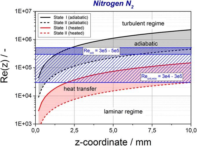
Mater. Res. Express 8 (2021) 036513                                                                    M Borkmann et al

   Figure 1. Schematic illustration of the laser beam fusion cutting process.

with dominant shear stress or pressure gradient effects on material removal. A conducted stability analysis of
their dynamic melt ejection model revealed instabilities for a pressure gradient controlled melt removal, and it
was argued that these instabilities correlate with ripple formation patterns on the cut edge surface. Olsen [19]
stated that heat flow fluctuations through the molten layer cause corresponding fluctuations in local melt front
velocities. Being located at the side of the kerf, those fluctuations will result in cut width variations, which will be
identified as striations of the resultant cut edge. It was also suggested that material evaporation in the lower
central part of the kerf is able of forcing the melt partially to the sides and reduces in this way the cut quality.
Schulz et al [20] described the dynamical behavior of the laser beam fusion cutting process in terms of the
evolving cutting kerf and the melt flow as a free boundary problem by use of integral methods. In particular, the
formation of the ripples of first kind without noticeable re-solidified materials is discussed in detail. They
concluded that the time-dependent movement of the width of the cutting front as a response to unavoidable
fluctuations of the processing parameters causes the onset of ripple formation at the cut edges. Hirano and
Fabbro [21] gave a detailed overview over the several types of mechanisms that have been so far theoretically
suggested to explain the striation generation in inert-gas steel cutting, including (i) external fluctuations of
operating parameters such as laser power and gas flow rate, (ii) hydrodynamic instabilities induced in the melt
layer during its interaction with the gas flow, and (iii) instabilities of the thermal dynamics. Hirano and Fabbro
[22, 23] also performed extensive experimental investigations on disk laser cutting stainless steel and identified
periodical generations and downward displacements of melt accumulations at the cut edges. Also the stability of
the central cut front melt flow was discussed as a factor for the final surface roughness. Other experimental
studies applied the so-called trim-cut technique to visualize the melt flow under approximated cutting-like
conditions. Yudin and Kovalev [24, 25] revealed by corresponding high-speed camera observations that the
primary part of the melt flows down at the kerf sides in strokes, rivulets and droplets in a certain distance to the
cutting front. Ermolaev et al [26] performed comparative trim-cut trials with CO2 and fiber laser radiation and
indicated fundamental differences in the process characteristics. A very comprehensive overview of the different
stages of the development of the trim-cutting technique was recently given by Arntz et al [27–29] who used this
technique to analyze the melt flow dynamics in fibre laser cutting and demonstrated a possible impact of
multiple reflections on striation formation. Recently the melt ejection and dross formation at the bottom side of
the kerf was investigated by Stoyanov et al [30] and Pacher et al [31].
    The mentioned experimental investigations brought very interesting insights into the dynamics of striation
formation. However, underlying cause-effect relationships remain far from being fully understood. In
particular, the role of the cutting gas flow and its impact on the development of the final striation pattern on cut
edges remain vague. Recent results on fiber laser cutting stainless steel by Borkmann et al [32] revealed a
surprisingly close correlation between measured roughness values and computed characteristics of simulated
cut edge shear stress distributions. Consequently, it seems to be worthwhile to immerse deeper into
investigations about the possible influence of gas flow dynamics on the observed complex cut edge topography.
    Research on gas flow aspects in laser fusion cutting with high-pressurized gas jets also has already a long-time
history. Fieret et al [33] already gave a comprehensive overview of the underlying physics, the structure of free
gas jets and the influence of various nozzle types on the resultant flow distribution. Vicanek and Simon [34]
developed a theoretical model to evaluate the forces of the gas jet on the molten layer under laser cutting
conditions. They concluded from their calculations that the blow out of the melt is a result of two driving effects,
namely the pressure gradient and the shear stress due to friction, both being found of the same order of
magnitude. Petring et al [35] experimentally investigated the flow structure in free gas jets as well as in
interaction with transparent model kerfs by means of the Schlieren technique. They described the structure of
the supersonic flow within the kerf and pointed out that the interaction between the core gas flow and the

                                                          3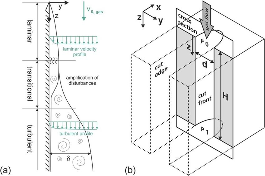
Mater. Res. Express 8 (2021) 036513                                                                                      M Borkmann et al

   Figure 2. Schlieren visualization of the flow through a transparent cut kerf model of 20 mm depth and 1.5 MPa gas pressure (a), and
   simulation of the core gas flow field with corresponding boundary conditions (b).

boundary layer might influence the melt flow and result in instabilities causing irregular cut edge structures.
Zefferer et al [36] linked the detected shock structures of the gas flow within modelled kerfs to distinct and
horizontally aligned lines commonly observable at standard CO2 laser cut edges. They also investigated the
influence of gas pressure and nozzle type on the position of the so-called boundary layer separation point, i.e. the
location where the core flow is found to be separated from the cut front or edge boundary. This macroscopic
flow phenomenon is usually considered of being responsible for a clearly observable melt ejection failure in laser
fusion cutting that gives rise to recast and dross problems at the base of the cut [37, 38]. Over the time, also many
experimental and numerical investigations were conducted on the performance of different nozzle types, e.g. by
Masuda and Moriyama [39], Man et al [40], and Kovalev et al [41]. A very comprehensive review on the influence
of the cutting gas flow on characteristics in laser beam fusion cutting was recently compiled by Riveiro [42].
Discussed are (i) the macro structure of the supersonic gas jet as a free stream as well as in interaction within cut
kerf models, (ii) the role of the boundary layer separation point for melt removal, and (iii) the influence of
different nozzle types on the efficiency of melt removal. They concluded that the interaction between gas and
molten film is of vital importance and that advanced CFD simulations and new theoretical and experimental
approaches are required to deepen the understanding of corresponding effects.
    Because the numerical efforts for advanced CFD simulations are thought of being immense for
corresponding simulations, this work is initially dedicated to an analytical characterization of the principal
properties of the developing boundary layer at cut edges under conditions of a high-pressurized cutting gas flow
through a narrow kerf. It will give first estimations about the expected boundary layer flow state, the relevant
factors that cause the transition from a laminar into a turbulent regime, the boundary layer thickness, as well as
characteristic numbers for momentum and heat transfer. As a result, this analysis will provide data that might be
useful for an adequate modelling and numerical simulation of the gas boundary layer in laser fusion cutting to
resolve its particular spatial and temporal flow structure.

2. Physical description of the cutting gas flow

As already mentioned, in laser fusion cutting a high-pressure inert gas is coaxially arranged to the laser beam to
eject the molten material. Commonly, nitrogen at pressures between 0.5 and 2.0 MPa is used as a cutting gas. In
general, the diameter of the mainly applied conical nozzles clearly exceeds the width of the cut kerf and especially
at low nozzle-material distances up to 1.0 mm almost constant gas conditions result at the nozzle center.
The ratio of the gas pressure to the ambient pressure clearly exceeds the critical pressure ratio of 1.89 and a
supersonic gas jet is formed. Figure 2(a) depicts a Schlieren picture of a flow through a cut kerf model made of
glass to reveal its macrostructure under adiabatic conditions of non-heated, i.e. cold surfaces.
     Due to the high pressure ratio the gas is massively expanded and accelerated. The gas flow exceeds sonic
speed and a complex 3D structure of compression shocks and expansion fans develops. In figure 2(b) a
simulated velocity distribution under consistent boundary conditions according to figure 2(a) is shown. The
commercial CFD-Code FLUENT and Reynolds-averaged-Navier–Stokes equations with an appropriate
turbulence model and standard wall functions were used in the simulation. A detailed description of the

                                                        4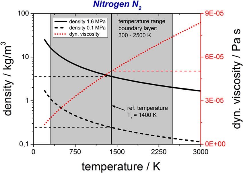
Mater. Res. Express 8 (2021) 036513 M Borkmann et al
Figure 3. Development of the boundary layer from a laminar to a turbulent flow state adopted from [43] (a) and 2D channel model of
the cutting gas flow through the cut kerf (b).
numerical model can be found in [32]. Obviously, the simulation results show a high level of agreement with the
experimentally recorded flow distribution, and it can be concluded that the gas flow simulation provides reliable
results. The detected gas flow separation at the cut front, as clearly recognizable in the experimental and
numerical results as well, was already linked to a macroscopic melt ejection failure in practical laser fusion
cutting experiments causing increased amounts of recast and dross at the base of the cut. Then again, the
macrostructure of the gas flow is however not capable of resolving the flow structure within the gas boundary
layer that might play a vital role for the cut edge topography.
3. 2D channel model of the cutting gas flow
The formation and development of a boundary layer (BL) by a fluid flowing over a solid surface has been a
subject of intensive fundamental and applied research for decades [43]. Figure 3(a) schematically shows the
development of the BL from a laminar into a turbulent state for the case of a fluid flow over a flat surface and a
turbulent core flow. At first, the BL is very thin and laminar. At some distance z to the leading edge, conditions
are changing by developing instabilities. The BL becomes turbulent with high mixing grades normal to the wall
and the BL dramatically grows in thickness. The transition process and the ongoing production of turbulence
within the boundary layer are governed by large scale coherent vortex structures which affect the local
distributions of shear stress and heat flux at the wall. Semi-empirical equations are available which allow
predictions about the flow state (laminar vs. turbulent) of the BL, as well as a quantification of corresponding
momentum and heat transfer rates.
For this purpose and in first approach, the complex three-dimensional gas flow in laser fusion cutting is
approximated by a 2D channel model with vertical cut edges as shown in figure 3(b). The assumption of parallel
side walls is supposed to be applicable in the case of larger material thicknesses and less focused laser beams.
Despite its simplicity, it is expected by the authors that fundamental and general findings about the boundary
layer development can be drawn. The 2D model geometry relies on the definition of a cross section of the kerf at
the junction of the front and side walls. It is defined by a constant distance d=0.8 mm between the parallel walls
and a height H=10 mm that corresponds to an exemplary sheet thickness separated by means of laser fusion
cutting.
Nitrogen as the preferred gas in laser fusion cutting is considered as an ideal gas with the specific gas constant
RN2=296.8 J/(kg K). The flow velocity and pressure at the inflow boundary are considered of being constant.
This assumption can be well justified by the fact that the diameter of the used gas nozzles in laser fusion cutting is
typically much larger than the kerf width. Furthermore, the estimation also requires a constant flow rate through
the kerf over the entire kerf depth. Two limiting flow states are evaluated to cover the entire range of conceivable
gas states in laser fusion cutting as extracted from gas flow simulations of the core gas flow under cutting
5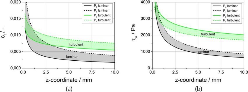
Mater. Res. Express 8 (2021) 036513 M Borkmann et al
Table 1. Reference values of for the defined flow states P0 (state I) at the top of
the kerf and P1 (state II) at the outlet.
Quantity Symbol Dimension State I State II
Pressure P MPa 1.6 0.1
Velocity u m s−1 200 600
Density ρ kg m−3 18.4 1.15
Viscosity η Pa s 16.8×10⁻⁶ 16.8×10⁻⁶
conditions as shown in figure 2(b). The first flow state (State I) is defined by the inflow condition at the top of the
kerf with high gas pressure P0 and a high but still subsonic velocity u. The second flow state limit (State II) relies
on the outflow condition with the pressure P1 at the outlet of the channel that roughly corresponds to the
ambient pressure and a supersonic velocity corresponding to a Mach number of Ma=2. Related boundary
conditions and gas properties are listed in table 1. Here, the density values are calculated according to the general
gas equation of ideal gases:
P
r N2 = (1)
RN2 · T
for a reference temperature of 293 K. The reference value of the dynamic viscosity was borrowed from gas
property tables given by Jeschar et al [44].
Using the given values, the Reynolds number as the principal dimensionless number of the similitude theory
to characterize the state of a flow can be calculated for the core flow according to its definition as ratio of inertial
to viscous forces:
u·r·d
Re d = (2)
h
with the flow velocity u, the gas density ρ, the kerf width d as characteristic length and the dynamic viscosity η. A
Reynolds number value of Red,crit≈2300 is typically given as a critical value for a transition from a laminar into
a turbulent flow regime for tube and channel flows. Both of the defined flow conditions at the inlet and the outlet
of the kerf lead to Reynolds numbers that are much larger than this threshold value. In case of the inlet (State I)
one gets Red,P0=1.75×10⁵, and for the outlet (State II) a Reynolds number of Red,P1=3.3×10⁴ is
calculated. Thus, the channel core flow will be of turbulent nature.
Most interesting for an evaluation of the developing boundary layer at the cut edge are its flow state and
thickness, as well as estimations of the expectable momentum and heat transfer rates between edge surface and
gas. Due to the fact that the edge surface is strongly heated under cutting conditions by the incident laser beam,
the analysis is principally performed under conditions of a heated and high-temperature wall.
The flow state of the boundary layer and its thickness are dependent on the local position z along the
overflowed surface (figure 3(a)). Respectively, the Reynolds number of the boundary layer Rez is not defined for a
constant value of a characteristic length like the Reynolds number Red of the core flow but depends on the
position z along the overflowed solid surface:
u · r (T , p ) · z
Re z = f (z ) = (3)
h (T )
A critical value Rez,crit≈3×10⁵–5×10⁵ is reported for the transition to a turbulent state for the flow over a
flat plate with sharp leading edges. In case of an unshapely leading edge as it might be more characteristic in laser
fusion cutting, the critical Reynolds number can be even reduced to a critical value of Rez,crit,min≈3×10⁴.
Due to the thermal nature of the cutting process also a thermal boundary layer develops which in turn affects
the boundary layer flow as a result of the inherent heat transfer between the cold gas and the hot cut edge surface.
The temperature of the liquid melt layer in laser fusion cutting must be lying between the melting and boiling
point of the material, i.e. between 1800 K (1530 °C) and 3000 K (2730 °C) in case of iron or ferrous alloys,
respectively. To facilitate the analysis, an average and constant value of 2500 K (2230°C) is assumed for the whole
cut edge surface. The assumption of this value of temperature magnitude is not only justified by the empirical
process understanding but also by experimental temperature measurements of the cut front interface during
laser fusion cutting of stainless steel [45]. Such a thermal boundary condition causes a temperature distribution
throughout the boundary layer with a gas temperature of 2500 K at the wall, i.e. cut edge surface, and the
temperature of the core flow (roughly ambient temperature, i.e.≈300 K) at the outer edge of the thermal
boundary layer. In such a case, the temperature dependence of density and viscosity can play an important role
for the boundary layer development and must be considered [46]. Calculated values of the density as a function
of temperature and pressure according to the state equation of ideal gases, as well as values of the dynamic
6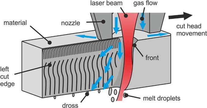
Mater. Res. Express 8 (2021) 036513 M Borkmann et al
Figure 4. Density and viscosity of nitrogen versus temperature. Densities values are calculated for both reference pressures according
to equation (1).
viscosity as a function of temperature according to a power approach given again by Jeschar et al [44] are shown
in figure 4.
Because the thermal boundary layer thickness of gases with Prandtl numbers Pr = n /a » 1 (ratio of
kinematic viscosity n to thermal diffusivity a ) is similar in magnitude to the thickness of the flow boundary layer,
it seems to be sufficiently justified to assume an average reference temperature of Tref=1400 K to characterize
the thermal state of the flow boundary layer. With this assumption, boundary layer Reynolds numbers can be
calculated as a function of the position along the kerf surface according to equation (3).
A very important quantity of the boundary layer that can be calculated as a function of the resulting Reynolds
number values Rz is the thickness δ of the boundary layer. Distinguishing between laminar and turbulent flow
regimes, Schlichting and Gersten [43] recommended the following approximations:
d lam (z ) = 5.0 · z · Re-
Z
0.5
(4)
d turb (z ) = 0.37 · z · Re-
Z
0.2
(5)
The local momentum transfer between cut kerf edge and gas flow that plays the most crucial role with regard to
the blow out of molten material in real fusion cutting experiments, also depends on the boundary layer flow
state. Corresponding shear stresses can be calculated as a function of local friction coefficients cf (z). Introducing
the friction coefficient functions as derived for a flow over a plane surface by Schlichting and Gersten [43], one
gets the following equations for the wall shear stresses τW,lam and τW,turb in case of laminar and turbulent
boundary layer flow states:
r
tW ,lam (z ) = c f ,lam (z ) · pdyn = 0.664 · Re-
z
0.5
· 2
· u¥ (6)
2
r
tW ,turb (z ) = c f ,turb (z ) · pdyn = 0.0592 · Re-
z
0.2
· 2
· u¥ (7)
2
The heat transfer rates between the gas and the cut edge surface can be estimated by applying well-known
equations for the Nusselt number Nu as a function of boundary layer Reynolds number Rez and the Prandtl
number Pr. To facilitate the analysis, only mean values over the overall flow length, i.e. the kerf height H=10
mm, are calculated. Corresponding equations are given by Baehr and Stephan [47] for the case of a flow over a
plate. Under conditions of a laminar BL, the corresponding relation for the Nusselt number can be analytically
derived:
NuMean,lam = 2 · Nu (z = H ) = 0.664 · Re1z/=2H·Pr1 / 3 (8)
In case of a turbulent BL, an empirical correlation equation by Gnielinski [48] is recommended. It reads as
follows:
7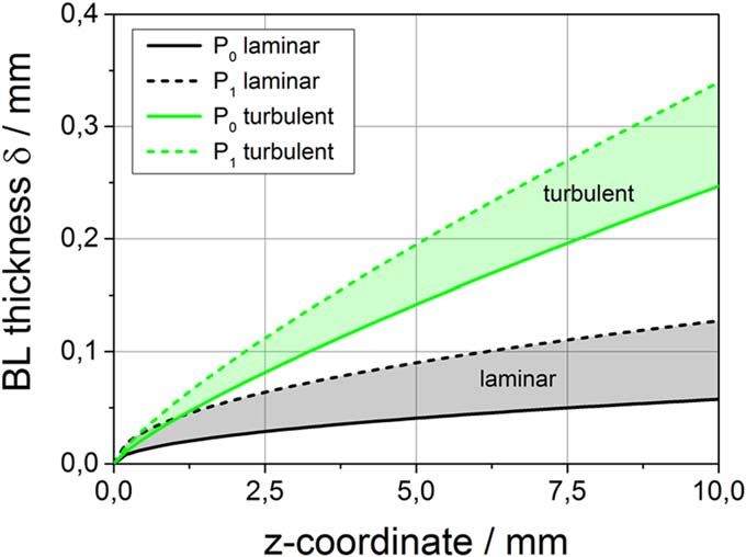
Mater. Res. Express 8 (2021) 036513 M Borkmann et al
Figure 5. Local boundary layer Reynolds number for the different cases of an adiabatic (Twall = Tref,gas = 300 K) and a heated wall
(Twall = 2500 K, Tref,gas = 1400 K ) with consideration of temperature-dependent gas properties. Transition zones according to
critical Reynolds number limits are shaded.
0.037 · Re0.8 · Pr
NuMean,turb = (9)
1 + 2.443 · Re-0.1 · (Pr 2 / 3 - 1)
The heat transfer for transitional states of the boundary layer is then considered as a mixed regime and the
corresponding Nusselt number can be approximated by a quadratic blending function:
NuMean,tran = Nu2Mean,lam + Nu2Mean,turb (10)
The given equations allow an estimation of the heat transfer coefficient αMean according to the definition of the
Nusselt number:
1
aMean =
· NuMean · lN2 (11)
H
with λN2 as the heat conductivity of nitrogen. Assuming that the kerf front can be considered of being a half
cylinder with a diameter d that corresponds to the kerf width d and a height H, the overall heat flux Q from the
heated front surface to the gas flow follows to:
d
Q = qmean · Afront = amean (Tw - TG ) · p · · H (12)
2
with the heat flux density qMean, the front area Afront , the wall temperature Tw and the core gas temperature TG.
With this set of semi-empirical equations, tentative estimations of the BL flow state, BL thickness and
momentum and heat transfer can be prepared for the gas flow in laser fusion cutting under the mentioned
assumptions.
4. Results and discussion
4.1. Boundary layer flow state and thickness
Boundary layer Reynolds numbers Rez can be calculated as a function of the position along the kerf surface
according to equation (3). Figure 5 shows the resultant dependencies for an adiabatic (Twall = Tref,gas = 300 K )
and a strongly heated surface (Twall = 2500 K, Tref,gas = 1400 K ) in graphical context with the mentioned
critical Reynolds numbers Rez,crit and Rez,crit,min. It becomes clear that the consideration of the thermal state of
the boundary layer strongly affects the position at which the laminar boundary layer is prone to turn into a
turbulent stage. In case of a cold material (or an adiabatic wall), the transition already occurs at the top of the
kerf. At about z=2 mm, the defined critical Reynolds number range is exceeded and a turbulent flow boundary
layer is predicted for the remaining kerf region. In contrast, if the heat transfer to the gas is considered—and that
might be regarded as realistic condition with respect to laser fusion cutting—the predicted state of the flow
boundary layer changes: Due to the decrease of the density and the increased viscosity at elevated temperatures,
the corresponding Reynolds numbers of the BL are decreased by more than one order of magnitude. In that case,
the Reynolds number is initially well below the minimum critical value of Rez,crit,min and at least the upper 2 mm
of the BL are predicted of being in a laminar state. This means that this part of the BL is stable and perturbations
should be attenuated. For higher depths, the calculated Reynolds numbers still remain in the lower range of the
8Mater. Res. Express 8 (2021) 036513 M Borkmann et al
Figure 6. Local boundary layer thickness for laminar and turbulent states of the heated boundary layer. Heat transfer and temperature
dependent gas properties are considered.
Figure 7. Local friction coefficient (a) and local wall shear stress (b) as a function of z-coordinate for different flow conditions.
critical zone and the flow state is potentially transitional between the laminar and the turbulent flow regime.
Although the BL might become unstable and perturbations will probably no longer effectively be attenuated, it is
probable that the amplification of disturbances remains small due to the moderate Reynolds numbers. In any
case, the length of the transition process to a fully turbulent flow state will be enlarged.
Calculated values of the boundary layer thickness δ for laminar and turbulent flow states for the relevant case
of a heating wall are displayed in figure 6. For the sake of simplicity, it is assumed that the turbulent BL is also just
starting at the upper corner of the channel edge.
It is obvious that the thickness of the turbulent BL grows much faster than that of the laminar BL. At z=
10 mm a turbulent BL reaches a thickness of 250 μm to 340 μm whereas a laminar BL is predicted of being only
60 μm to 120 μm thick. That means that the boundary layers of the opposite cut edges of an assumed kerf width
of 800 μm are not supposed to meet each other over the considered height H of the kerf, i.e. the assumption of
independent opposite boundary layers is justified. Furthermore, analogy approximations of the well investigated
case of a flow over a flat plate—as given in the model description - are applicable for a characterization of related
coefficients of momentum and heat transfer.
4.2. Momentum and heat transfer
Calculated local friction coefficients and resultant local wall shear stress values according to equations (6) and (7)
are depicted in figure 7 for the both limiting flow states and a heated wall as a function of the z-coordinate.
Comparable shear stress values for the laminar and turbulent flow state in the range of 3000–4000 Pa are
prognosticated for the top part of the channel for z1 mm only. For higher z-values, the magnitudes of wall
shear stress become clearly distinguishable. In consistence with theoretical expectations, the values of friction
9Mater. Res. Express 8 (2021) 036513 M Borkmann et al
Figure 8. Calculated heat transfer rates between front wall and gas for different boundary layer flow states and different boundary
conditions.
coefficient and wall shear stress are larger for a turbulent state of the boundary layer. It is worthwhile to
emphasize the fact that the estimated wall shear stresses—despite the large pressure and density differences
between the both considered limiting flow states—are primarily influenced by the boundary layer flow state.
Correspondingly, the calculated value ranges appear as well-distinguishable narrow bands for the laminar and
turbulent BL flow state. The calculated high shear stress values at the top of the kerf dramatically decrease
downwards within the first 2 mm with a steeper loss of shear stress magnitude in case of the laminar BL. For
larger z-coordinates, the shear stress of a turbulent BL is approximately twice as high as for a laminar BL. In the
region of the defined outlet for z=10 mm, a laminar BL generates shear stresses of 800 Pa, whereas a turbulent
BL is still capable of exerting up to 2000 Pa. These calculated shear stress values correspond very well to
numerically computed maximum axial shear stress values of a cutting gas flow CFD analysis [32].
Calculated values of heat flux density q Mean and overall heat flux Q are shown in figure 8 for the different
boundary layer flow states under consideration of the limiting boundary conditions. Apparently for all flow
states, the heat transfer for the gas condition at the top of the kerf is more than twice as intensive as the one for the
bottom condition. Hence, a notably higher heat transfer at the entrance region of the kerf can be expected.
Furthermore, for a transitional or turbulent boundary layer, the heat transfer is doubled in comparison to
laminar boundary layer conditions. For the used value of an averaged cut front temperature of about 2200 °C a
total heat transfer loss of 24–114 W is estimated. In conventional laser fusion cutting, e.g. with 4 kW laser power
for cutting of 10 mm stainless steel and an experimentally determined coupling efficiency of about 50% [49] this
loss corresponds to less than 3% of the applied laser power or to less than 6% of a absorbed laser power,
respectively. These contributions seem to be insignificant.
5. Summary
In laser fusion cutting the combined action of laser beam and inert cutting gas flow produces a 3D cut kerf
geometry with locally varying kerf width and front inclination. The applied high pressure supersonic gas jet is
characterized by a complex 3D flow structure of compression shocks, expansion fans and there interactions.
After decades of industrial application and scientific investigations the involved physical mechanisms especially
concerning the melt driving forces are still not fully understood. Since the interface between gas and melt flow is
crucial for the acceleration and removal of melt this work gives tentative estimations of basic gas boundary layer
properties. The developed analytical 2D model for the gas flow in laser fusion cutting is based on the following
assumptions and approximated flow conditions:
• 2D channel model with parallel walls, 10 mm in length and 0.8 mm in width
• constant base flow conditions along the channel, i.e. pressure chances and acceleration of the gas are
disregarded
• consideration of flow condition state I (inflow at high pressure and low velocity) and state II (outflow at
ambient pressure and supersonic velocity) as approximate thresholds of the actual flow
10Mater. Res. Express 8 (2021) 036513 M Borkmann et al
• adiabatic wall or constant wall temperature of 2500 K
• Nitrogen as ideal gas with density, pressure and temperature according to general equation of state and
temperature dependent viscosity according to Jeschar et al [44]
The assumptions made allow for the applicability of the semi-empirical equations and relationships from the
similitude theory.
The study revealed that the heat transfer from the wall to the cutting gas has a crucial impact on the gas
boundary layer flow state and its development along the cutting front and cut kerf edge, respectively. In an
adiabatic case with constant gas properties at ambient temperature, an almost completely turbulent boundary
layer is predicted with an early transition to a turbulent state at the top of the kerf. In contrast, if more realistic
thermal boundary conditions and temperature-dependent gas properties are considered, the boundary layer is
initially found to be laminar and becomes susceptible for perturbations just after some millimeter distance from
the leading edge. But the analysis also suggests that the transition process to a turbulent flow regime is very
elongated with weak amplification of instabilities.
Subsequently, the estimations of derived quantities like boundary layer thickness, wall shear stress and heat
transfer differ between the principal flow states. For a completely turbulent boundary layer a thickness of up to
340 μm is predicted whereas a laminar boundary layer is just 120 μm thick after 10 mm flow over the surface or
cut edge, respectively. The presumed transitional boundary layer is thought to be in between but only slightly
larger than the laminar case due to the attenuation or weak amplification of instabilities. For all BL flow states
shear stresses higher than 3000 Pa are estimated for the first millimeter of cut edge. The area of high shear stresses
corresponds well to the uppermost section at the cut edge where striations as depth variation of the base material
without resolidified melt were described by Zefferer [14] and Borkmann et al [17]. Considering that high shear
stresses facilitate an effective removal of the melt this coincidence seems to be expectable. The current BL flow
state is especially essential for the calculated local shear stresses for material thicknesses over 2 mm. The average
momentum transfer at z=10 mm for a transitional or turbulent BL reaches values up to 2000 Pa and is twice as
large as the shear stress of a laminar flow state. An effect of the BL flow state is also seen with respect to
prognosticated heat transfer rates. Additionally, an even more pronounced effect of the base flow conditions is
detected. Higher heat flux rates are found at the top of the kerf and a decrease of local heat flux rates with
increasing z-coordinate is expected. Nevertheless, both the estimated heat flux densities and the overall heat flux
values are relatively small and should be negligible in comparison to the intensities and powers of high-power
laser beams usually applied and absorbed in thick-section metal sheet cutting.
6. Conclusions
At least for two different scopes sweeping conclusions can be drawn from the results of this study. The first one
concerns the modelling and simulation of laser cutting processes. Despite of sophisticated models for absorption
and reflection of the laser beam, resulting temperature distributions, the melting of the material and the melt
flow, commonly the gas flow is highly simplified in processing models, e.g. to low velocities, reduced to a
simplistic boundary condition derived from analytical assumptions or even disregarded at all. Actually this work
emphasizes the strength of impact and possible variety of gas flow features and boundary layer development
even for a gas model at this high level of simplicity. Hence some recommendations concerning gas flow
consideration for more realistic modelling and simulation of laser cutting processes can be given:
• realistic boundary conditions for pressure and temperature
• modelling of viscous terms and resolution of boundary layer development
• temperature dependent gas material properties
Considerably, as a result of this analysis it can be concluded that an engagement with the characteristics of
gas flow and boundary layer development in modelling of laser fusion cutting has the potential to upgrade the
level of process understanding.
A second application area is the analysis and interpretation of experimental cut edge structures. Commonly
the cut edge topography is considered as result of an inherent instability of the melt flow. Proceeding from the
present work an alternative interpretation by means of boundary layer development is reasonable. It is
worthwhile to note that the roughness values RZ (average height difference between the highest peak and the
lowest valley) of good quality fiber or disk laser cuts in stainless steel sheets with a thickness of 10 mm are
typically lying in a range of between 30 and 60 μm in dependence on the distance of the actual measurement
position to the top edge. Thus, it can be concluded from the performed analysis that the interaction between
11Mater. Res. Express 8 (2021) 036513 M Borkmann et al
Figure 9. High resolution microscopic picture of a good quality cut edge for fiber laser cutting in 10 mm stainless steel and detail from
the bottom half in true color and as elevation map.
melt film and gas as well as the formation of the particular structure of the cut edge clearly takes place within the
boundary layer region. The fact that a transitional boundary layer with a weak amplification of instabilities is
predicted has a far-reaching impact on structure and development of the boundary layer. During the transitional
flow state coherent vortices develop in the BL in consequence of the instability of the BL. These vortices govern
momentum and heat transfer at the wall and lead to growing average shear stresses and heat flux densities. It has
to be considered that the presented analysis only provides integral estimations of the expectable magnitudes of
the calculated quantities. Actual local distributions of shear stress and heat flux at cut edge surfaces will be
strongly affected by characteristics of the boundary layer development under process conditions of narrow and
inhomogeneously heated kerf surfaces and high spatial pressure and velocity gradients of the core flow. Thereby,
as proven by experimental investigations, the local transitional heat flux and shear stress can overshoot turbulent
values up to 50% [50] due to the high degree of regularity of the vortex structure in the transitional BL. Highly
expectable is a strong impact of the processing conditions in laser cutting on the kind of evolving instability
modes and corresponding vorticity properties and hence on the actual local distributions of shear stress and heat
flux [51–53].
Due to a lengthy transitional boundary layer with weak amplification, coherent vortices of primary and
secondary instability modes probably have abundant opportunities to imprint their structure into resolidifying
melt remains due to locally varying shear stresses and heat fluxes. Especially in case of stationary respectively
non-moving vortices it should be possible to draw inferences from the cut edge structure about the vortex
structure of the boundary layer. In figure 9 a high-resolution microscopic picture of a good quality cut edge for
fiber laser cutting in 10 mm stainless steel and a detailed view of the bottom part in true color and as elevation
map are shown. The whole cut edge is characterized by a very regular pattern of almost vertical striations. Within
the first millimeter at the top the horizontal wavelength of the striations is very small and about 125 μm.
Towards the bottom the wavelength increases to about 200–300 μm but is still very regular. In the detailed view
from the bottom half and the elevation map spirally shaped heaps lined up at one side of the striations are clearly
12Mater. Res. Express 8 (2021) 036513 M Borkmann et al
identifiable. Notably at the left kerf side they are located at the right side of a striation crest and rotate
anticlockwise inwardly while at the right kerf side the location and behavior are inverse. Anticipating that the cut
edge topography results as imprint of the boundary layer vortex structure these experimental findings show a
high resemblance to primary and secondary instability modes of a crossflow instability, e.g. numerically
determined by Bonfigli and Kloker [54]. Prospectively, the interpretation of the resultant cut edge by means of
boundary layer development at least should broaden existing explanation approaches.
Acknowledgments
The work was in parts financially supported by the German Research Foundation DFG within the project
‘Evaluierung dynamischer Lösungsansätze zur Optimierung des Inertgasschneidens von Dickblech mit
Laserstrahlquellen hoher Strahlqualität’, Contract No. BE1875/36-1. This support is highly appreciated by the
authors.
Data availability statement
All data that support the findings of this study are included within the article (and any supplementary files).
ORCID iDs
M Borkmann https://orcid.org/0000-0002-1182-0245
A Mahrle https://orcid.org/0000-0001-9190-6999
References
[1] Powell J 1998 CO2 Laser Cutting 2nd edn (Berlin: Springer)
[2] Powell J, Petring D, Pocorni J and Kaplan A 2017 LIA Guide to High Power Laser Cutting 1st ed. (Orlando, FL: Laser Institute of
America)
[3] Schuöcker D 1986 Dynamic phenomena in laser cutting and cut quality Appl. Phys. B 40 9–14
[4] Petring D, Schneider F, Wolf N and Nazary V 2008 The relevance of brightness for high power laser cutting and welding Proc. of the 27th
Int. Congress on Applications of Lasers & Electro-Optics, ICALEO 2008, Temecula (CA, USA), Laser Materials Processing Conference
95–103
[5] Mahrle A, Bartels F and Beyer E 2008 Theoretical aspects of the process efficiency in laser beam cutting with fiber lasers Proc. of the 27th
Int. Congress on Applications of Lasers & Electro-Optics, ICALEO 2008, Temecula (CA, USA), Laser Materials Processing Conference
703–12
[6] Petring D 2009 Calculable laser cutting Proc. of the Fifth Int. Conference on Lasers in Manufacturing, LIM 2009, Munich (Germany)
(June 15th–18th) 209–14
[7] Mahrle A and Beyer E 2009 Theoretical aspects of fibre laser cutting J. Phys. D 42 1175507
[8] Mahrle A and Beyer E 2009 Theoretical estimation of achievable travel rates in inert-gas fusion cutting with fibre and CO2 lasers Proc. of
the Fifth Int. Conference on Lasers in Manufacturing, LIM 2009, Munich (Germany) (June 15th–18th) p 6
[9] Mahrle A and Beyer E 2009 Thermodynamic evaluation of inert-gas laser beam fusion cutting with CO2, disk and fiber lasers Proc. of
the 28th Int. Congress on Applications of Lasers & Electro-Optics, ICALEO 2009, Orlando (FL, USA) (November 2-5) Laser Materials
processing Conference 610–9
[10] Wandera C, Salminen A, Olsen F O and Kujanpää V 2006 Cutting of stainless steel with fiber and disk lasers Proc. of the 25th Int.
Congress on Applications of Lasers & Electro-optics, ICALEO 2006, Scottsdale (AZ, USA) 211–20
[11] Himmer T, Pinder T, Morgenthal L and Beyer E 2007 High brightness lasers in cutting applications Laser Materials Processing
Conference Proc. of the 26th Int. Congress on Applications of Lasers & Electro-Optics, ICALEO 2007, Orlando (FL, USA) (October 29–
November 1) 87–91
[12] Scintilla L D, Tricarico L, Mahrle A, Wetzig A, Himmer T and Beyer E 2010 A comparative study on fusion cutting with disk and CO2
lasers Proc. of the 29th Int. Congress on Applications of Lasers & Electro-Optics, ICALEO 2010, Anaheim (CA, USA) (September 26-30)
249–58
[13] Stelzer S, Mahrle A, Wetzig A and Beyer E 2013 Experimental investigations on fusion cutting stainless steel with fiber and CO2 laser
beams Phys. Procedia 41 392–7
[14] Zefferer H 1997 Dynamik des Schmelzschneidens mit Laserstrahlung Dissertation RWTH Aachen (Germany) Fakultät für
Maschinenwesen
[15] Hilton P A 2009 Cutting stainless steel with disc and CO2 lasers Proc. of the 5th Int. Congress on Laser Advanced Materials processing,
LAMP 2009, Kobe Convention Center (Kobe, Japan) (June 29–July 2) p 6
[16] Hu C, Mi G and Wang C 2020 Study on surface morphology and recast layer microstructure of medium thickness stainless steel sheets
using high power laser cutting J. Laser Appl. 32 022033
[17] Borkmann M, Mahrle A, Beyer E and Leyens C 2019 Cut edge structures and gas boundary layer characteristics in laser beam fusion
cutting Proc. of the Lasers in Manufacturing Conference, LIM 2019, Munich (Germany) (June 24–27) p 11
[18] Vicanek M, Simon G, Urbassek H M and Decker I 1987 Hydrodynamical instability of melt flow in laser cutting J. Phys. D 20 140–5
[19] Olsen F O 1994 Fundamental mechanisms of cutting front formation in laser cutting Laser material processing: industrial and
microelectronic applications Proc. of SPIE vol 2207, 402–13
13Mater. Res. Express 8 (2021) 036513 M Borkmann et al
[20] Schulz W, Kostrykin V, Nießen M, Michel J, Petring D, Kreutz E W and Poprawe R 1999 Dynamics of ripple formation and melt flow in
laser beam cutting J. Phys. D 32 1219–28
[21] Hirano K and Fabbro R 2011 Experimental investigation of hydrodynamics of melt layer during laser cutting of steel J. Phys. D 44 12
[22] Hirano K and Fabbro R 2011 Experimental Observation of hydrodynamics of melt layer and striation generation during laser cutting of
steel Phys. Procedia 12 555–64
[23] Hirano K and Fabbro R 2011 Study on striation generation process during laser cutting of steel Proc. of the 30th Int. Congress on
Applications of Lasers & Electro-Optics, ICALEO 2011, Orlando (FL, USA) (October 23-27) pp 50–9
[24] Yudin P and Kovalev O 2007 Visualization of events inside kerfs during laser cutting of fusible metal Proc. of the 26th Int. Congress on
Applications of Lasers & Electro-Optics, ICALEO 2007, Orlando (FL, USA) (October 29–November 1) pp 772–9
[25] Yudin P and Kovalev O 2009 Visualization of events inside kerfs during laser cutting of fusible metal J. Laser Appl. 21 39–45
[26] Ermolaev G V, Yudin P V, Briand F, Zaitsev A V and Kovalev O B 2014 Fundamental study of CO2 and fiber laser cutting plates with
high speed visualization technique J. Laser Appl. 26 9
[27] Arntz D, Petring D, Jansen U and Poprawe R 2017 Advanced trim-cut technique to visualize melt flow dynamics inside laser cutting
kerfs J. Laser Appl. 29 9
[28] Arntz D, Petring D, Stoyanov S, Jansen U, Schneider F and Poprawe R 2018 In-situ visualization of multiple reflections on the cut flank
during laser cutting with 1 μm wavelength J. Laser Appl. 30 032206
[29] Arntz D, Petring D, Schneider F and Poprawe R 2019 In situ high speed diagnosis—A quantitative analysis of melt flow dynamics inside
cutting kerfs during laser fusion cutting with 1 μ m wavelength J. Laser Appl. 31 022206
[30] Stoyanov S, Petring D, Arntz-Schroeder D, Günder M, Gillner A and Poprawe R 2020 Investigation on the melt ejection and burr
formation during laser fusion cutting of stainless steel J. Laser Appl. 32 022068
[31] Pacher M, Franceschetti L, Strada S C, Tanelli M, Savaresi S M and Previtali B 2020 Real-time continuous estimation of dross
attachment in the laser cutting process based on process emission images J. Laser Appl. 32 042016
[32] Borkmann M, Mahrle A and Beyer E 2018 Study of correlation between edge roughness and gas flow characteristics in laser beam fusion
cutting Procedia CIRP 74 421–4
[33] Fieret J, Terry M J and Ward B A 1987 Overview of flow dynamics in gas-assisted laser cutting Proc. of SPIE 0801 243
[34] Vicanek M and Simon G 1987 Momentum and heat transfer of an inert cutting gas jet to the melt in laser cutting J. Phys. D 20 1191–6
[35] Petring D, Abels P, Beyer E and Herziger G 1988 Werkstoffbearbeitung mit Laserstrahlung: Teil 10: Schneiden von metallischen
Werkstoffen mit CO2-Hochleistungslasern Feinwerktechnik und Messtechnik 96 364–72
[36] Zefferer H, Petring D and Beyer E 1991 Investigations of the gas flow in laser beam cutting Proceedings of the 3rd Int. Beam Technology
Conference Karlsruhe (Germany, March 13-14) 210–4
[37] Sparkes M, Gross M, Celotto S, Zhang T and O’Neill W 2006 Inert cutting of medium section stainless steel using a 2.2 kW high
brightness fibre laser Proc. of the 25th Int. Congress on Applications of Lasers & Electro-Optics, ICALEO 2006, Scottsdale (AZ, USA)
(October 30–November 2) 197–205
[38] Sparkes M, Gross M, Celotto S, Zhang T and O’Neill W 2008 Practical and theoretical investigations into inert gas cutting of 304
stainless steel using a high brightness fiber laser J. Laser Appl. 20 59–67
[39] Masuda W and Moriyama E 1994 Aerodynamic characteristics of underexpanded coaxial impinging jets, JSME International Journal,
Series B 37 769–75
[40] Man H C, Duan J and Yue T M 1997 Design and characteristic analysis of supersonic nozzles for high gas pressure laser cutting J. Mater.
Process. Technol. 63 217–22
[41] Kovalev O B, Yudin P V and Zaitsev A V 2008 Formation of a vortex flow at the laser cutting of sheet metal with low pressure of assisting
gas Journal of Physics D: Applied Physics 41 155112
[42] Riveiro A, Quintero F, Boutinguiza M, Val J D, Comesana R, Lusquinos F and Pou J 2019 Laser cutting: a review on the influence of
assist gas Materials 12 1–31
[43] Schlichting H and Gersten K 1997 Grenzschicht-Theorie, 9., Völlig Neubearb. (Springer-Verlag: Berlin Heidelberg)
[44] Jeschar R, Alt R and Specht E 1990 Grundlagen der Wärmeübertragung 3rd edn (Viola-Jeschar-Verlag)
[45] Onuseit V, Ahmed M A, Weber R and Graf T 2011 Space-resolved spectrometric measurements of the cutting front Phys. Procedia 12
584–90
[46] Severin J 1999 Der Einfluss der Wärmeübertragung auf die Stabilität von Strömungen, Dissertation Technische Universität Chemnitz
(Germany) Fakultät für Maschinenbau
[47] Baehr H D and Stephan K 2006 Heat and mass transfer (Berlin Heidelberg: Springer-Verlag)
[48] Gnielinski V 1975 Berechnung mittlerer Wärme- und Stoffübergangskoeffizienten an laminar und turbulent überströmten
Einzelkörpern mit Hilfe einer einheitlichen Gleichung Forsch. Ingenieurwes. 61 145–53
[49] Hügel H 1992 Strahlwerkzeug Laser (Stuttgart: Teubner Verlag)
[50] Morkovin M V 1991 Panoramic view of changes in vorticity distribution in transition instabilities and turbulence Proc. of the
Symposium on Boundary Layer Stability and Transition to Turbulence, Portland (OR, USA) (New York, June 23–27) (American Society of
Mechanical Engineers) 1–12
[51] Morkovin M V 1989 On receptivity to environmental disturbances ed M Y Hussaini and R G Voigt Instability and Transition: Materials
of the Workshop, Hampton (VI, USA) May 15–June 9) (New York(Springer)
[52] Arnal D and Casalis G 2000 Laminar-turbulent transition prediction in three-dimensional flows Prog. Aerosp. Sci. 36 173–91
[53] Saric W S, Reed H L and Kerschen E J 2002 Boundary-layer receptivity to freestream disturbances Annu. Rev. Fluid Mech. 34 291–319
[54] Bonfigli G and Kloker M 2007 Secondary instability of crossflow vortices. Validation of the stability theory by direct numerical
simulation J. Fluid Mech. 583 229–72
14You can also read