Latitudinal Gradient in Urban Pressure and Socio-Environmental Quality: The "Peninsula Effect" in Italy - MDPI
←
→
Page content transcription
If your browser does not render page correctly, please read the page content below
land
Article
Latitudinal Gradient in Urban Pressure and
Socio-Environmental Quality: The “Peninsula Effect”
in Italy
Bernardino Romano * , Lorena Fiorini , Chiara Di Dato               and Vanessa Tomei
 Department of Civil and Environmental Engineering, University of L’Aquila, 67100 L’Aquila, Italy;
 lorena.fiorini@univaq.it (L.F.); chiara.didato@graduate.univaq.it (C.D.D.); vanessatomei@gmail.com (V.T.)
 * Correspondence: bernardino.romano@univaq.it; Tel.: +39-862434113

 Received: 27 March 2020; Accepted: 22 April 2020; Published: 23 April 2020

 Abstract: The purpose of this work is to synthesize, for an international audience, certain fundamental
 elements that characterize the Italian peninsular territory, through the use of a biogeographical model
 known as the “peninsula effect” (PE). Just as biodiversity in peninsulas tends to change, diverging
 from the continental margin, so do some socio-economic and behavioral characteristics, for which
 it is possible to detect a progressive and indisputable variation depending on the distance from
 the continental mass. Through the use of 14 indicators, a survey was conducted on the peninsular
 sensitivity (which in Italy is also latitudinal) of as many phenomena. It obtained confirmation results
 for some of them, well known as problematic for the country, but contradictory results for others,
 such as those related to urban development. In the final part, the work raises a series of questions,
 also showing how peninsular Italy, and in particular Central–Southern Italy, is not penalized so
 dramatically by its geography and morphology as many political and scientific opinions suggest.
 The result is a very ambiguous image of Italy, in which the country appears undoubtedly uniform
 in some aspects, while the PE is very evident in others; it is probably still necessary to investigate,
 without relying on simplistic and misleading equations, the profound reasons for some phenomena
 that could be at the basis of less ephemeral rebalancing policies than those practiced in the past.

 Keywords: peninsula effect; urban pressure; south Italy; latitudinal gradient

1. Introduction
      This work is inspired by the biogeographical phenomenon known as the “peninsula effect” (PE)
to analyze and verify the influence of peninsular geography in Italy on various kinds of anthropic
activities, through a set of indicators aimed at highlighting environmental, social, and economic aspects
of this continental prominence that stretches for about 900 km in the Mediterranean Sea. These same
aspects are then investigated in parallel with the urban transformation of the soil which represents, in
Italy, one of the most serious pathologies affecting the quality of social life and biodiversity.
      The peninsula effect is a classic biogeographical concept which predicts that the number of
species declines from a peninsula’s basis to its tip. It is an extension of island theory, the subject of
experiments in multiple worldwide cases [1–6], on the basis of which there are significant differences
in the distribution and quantity/variety of biotic species along the peninsular area [7]. Two of the three
hypothesized causal mechanisms—the effects of geological history or habitat on species richness—can
be controlled for via the study design and/or statistical analysis. The third proposed mechanism
(reduced colonization towards the peninsular tip) is attributed to peninsular geometry and is less
easily controlled [8].
      The role of the PE can be at the basis of the well-known “southern question”; that is, the overall
socio-economic weakness of the south of the country, caused by the stratification of multiple historical

Land 2020, 9, 126; doi:10.3390/land9040126                                          www.mdpi.com/journal/land
Land 2020, 9, 126                                                                                       2 of 12

events [9–11], but which in the negative evolution of the last half century probably owes a lot to geographic
physiognomy and morphology. In this sense, some considerations can also be trivial, such as the extension
of land lines of communication to national and European economic gangs, the objective inefficiency
of maritime transport (historically much more important than today), and the design complexity of
non-coastal communications, due to the geomorphological harshness of the internal areas, especially
in the section of the Central Apennines. However, as is discussed in this paper, many contradictions
can be associated with this profile consolidated in common thought, which sees the dynamic of urban
transformation as an element capable of provoking questions and reversing convictions. The result is a
very ambiguous image of Italy, in which the country appears undoubtedly uniform in some aspects, while
the PE is very evident in others; it is probably still necessary to investigate, without relying on simplistic
and misleading equations, the profound reasons for some phenomena that could be at the basis of less
ephemeral rebalancing policies than those practiced in the past.

2. Data and Methods
      The measurement of the peninsula effect on various phenomena was carried out using a set of
14 indicators with values calculated on a regional basis. These indicators are derived from the initial
idea of comparing the differences along the peninsular arch that concern physical and social aspects
to bring out significant differences/homogeneities or links/contradictions. Therefore, research was
carried out on the data available at the same level of detail and recently updated for the whole national
territory in the demographic, urban, socio-economic, and environmental sectors, and the possibility
arose to fill in the 14 indicators used.
      For most of the indicators, the source used was ISTAT (Central Institute of Statistics), which
systematically publishes data relating to the population and the related economic and social components
at least every 10 years (but in many cases also more frequently). The data concerning quality and
environmental protection were instead derived from documents of the Ministry of the Environment or,
in the case of forests, from the European CORINE Land Cover 2012. Data from the urbanized areas
came from the processing carried out by the University of L’Aquila for the 1950s [12,13], while data for
the current period came from the digital land use maps developed by the regions until 2008 (LUM).
      More up-to-date and efficient data have been produced from 2015 onwards by the National
Environmental Research Institute (ISPRA) [14]. Monitoring occurs through the production of a
national land use map on a raster basis (regular grid), using data from Copernicus and, in particular,
the Sentinel-2 mission [15,16] launched in June 2015, which provides multispectral data with a 10-meter
resolution, suitable for both photo-interpretation and semi-automatic classification processes.
      For this study, we chose to use regional LUM data and not the ISPRA data updated in 2017, since
the latter also include surfaces covered by some categories of interurban roads (not separable) and
therefore cannot be compared with the 1950s data that did not include these elements. The urbanized
areas surveyed by ISPRA in 2017 exceed those of regional LUMs by approximately 260,000 ha. This
can be ascribed, in part, to the increase that has occurred over the past 10 years, but also largely to the
inclusion of the road network, amounting to almost 200,000 km out of the approximately 870,000 total
in Italy comprising all categories. It must be taken into account that the aspect of urbanization is one of
the most complex, as it presents significant typological differences, both within the Italian territory and
at the scale of the Mediterranean area [17–19]. In the case of the present research, the phenomenon has
been simplified and reduced to the four indicators defined to highlight the more macroscopic characters.
      The 14 indicators have been grouped into 5 categories: demographic (demographic density,
demographic variation rate, old age index), economic (average income, GDP per capita), social
(university degree, unemployment rate), environmental (protected area rate, Natura 2000 rate, forest
rate), and urban (urban density, urbanization per capita, urbanization variation rate, land take speed),
and their calculation was based on updated data in a chronological range between 2006 and 2011,
whose formulations and sources are indicated in Table 1.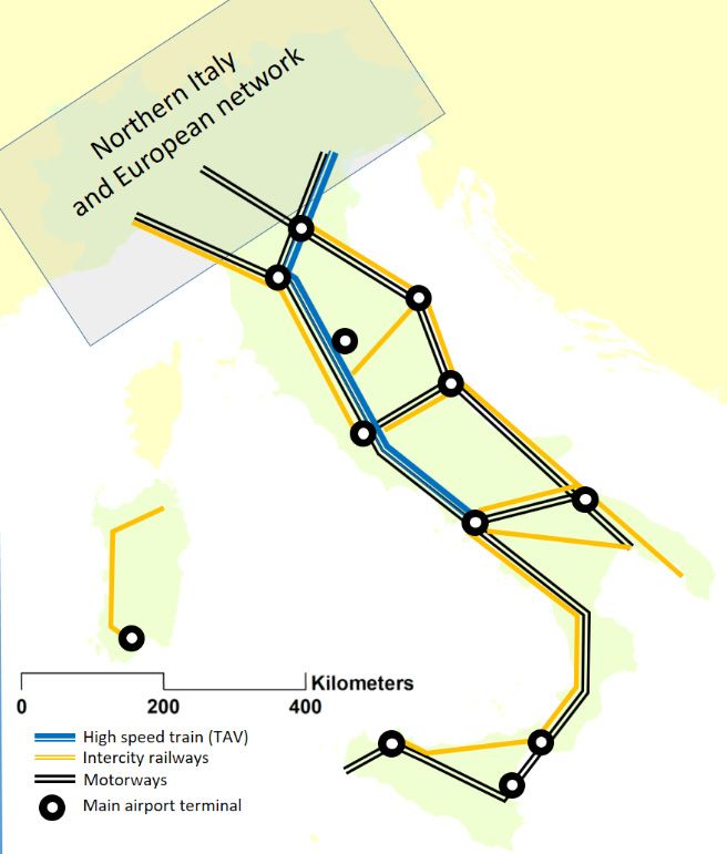
Land 2020, 9, 126                                                                                                                              3 of 12

                                                                     Table 1. Indicator set.

                                                                 Demographic indicators
                                                          p                      p= number of resident inhabitants
               Dd   Demographic density        Dd =                                                                       inhab/km2     2011
                                                          Ra                           Ra = Regional area
                                                                              p (2011)= population on 2011 (number of
                    Demographic variation           p(2011) −p(1950)                    resident inhabitants)
              Dvr                           Dvr =       p(1950)                                                              %        1950–2011
                           rate                                               p(1950)= population on 1950 (number of
                                                                                        resident inhabitants)
                                                          p>65                 p>65 = population older than 65 years
              OAi      Old Age Index          OAi =                                                                          %          2011
                                                          p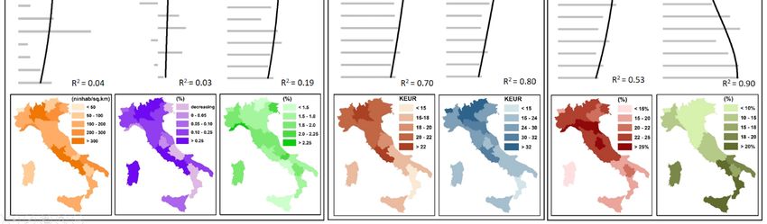
Land 2020, 9, 126                                                                                                                           4 of 12

                                                                            Table 1. Cont.

                                                                   Environmental indicators

                                                             PAa                   PAa = Regional protected areas area
              Par    Protected areas rate        PAr =                                                                     %         2018
                                                              Ra                          Ra = Regional area

                                                             N2ka                       N2ka = regional N2k area
             N2kr      Natura 2000 rate          N2kr =                                                                    %         2018
                                                              Ra                           Ra = regional area

                                                             Fa                         Fa = regional forest areas                 CORINE
               Fr         Forest rate                 Fr =                                                                 %
                                                             Ra                            Ra = regional area                       2018
                                                                       Urbanization indicators
                                                                                             Ua = urbanized areas
               Ud    Urbanization density         Ud =       Ua                                                          m2 /km2     2008
                                                             Ra                               Ra = regional area
                                                             Ua                           Ua= urbanized areas
              Upc   Urbanization per capita      Ud =                                                                    m2 /ab      2008
                                                           ninhabit.                 N(inhab) = resident inhabitants
                    Urbanization variation            Ua(2008) −Ua(1958)
              Uvr                             Uvr =       Ua(1950)                           Ua= urbanized areas           %       1958–2008
                            rate
                                                                                         Ua= urbanized areas
                                                      Ua(2008) −Ua(1958)
              LTs      Land take speed        LTs =         ndays
                                                                                 ndays = Number of days in considered    ha/day    1958–2008
                                                                                         time range (50 years)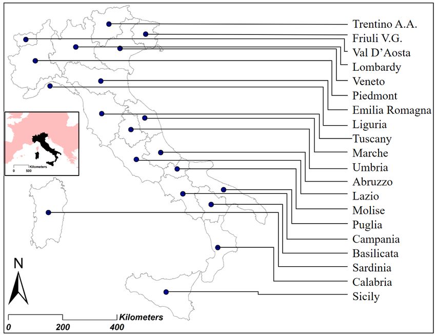
Land 2020, 9, x FOR PEER REVIEW                                                                                       3 of 12

speed),
Land 2020,and
           9, 126theircalculation was based on updated data in a chronological range between 20065 of                   and12
2011, whose formulations and sources are indicated in Table 1.
      The values assumed by the various parameters were then sorted by latitudinal succession from
northThe  valuesaccording
       to south     assumed by   to the
                                    the various    parameters
                                         geographical     locationwereof then   sorted by
                                                                         the regions       latitudinal
                                                                                       deduced     fromsuccession
                                                                                                          the position from
                                                                                                                          of
their centroids (Figure 1). The ordinal positioning of the data made it possible to verify the degree of
north  to south    according     to the  geographical     location    of the  regions  deduced     from   the  position   of
their centroids
sensitivity       (Figure
             of the          1). Thecorrelated
                     phenomena        ordinal positioning      of the
                                                  with latitude;       data
                                                                     and     made it trend
                                                                          therefore,  possible   to verify
                                                                                             curves          the degree
                                                                                                       of order           of
                                                                                                                  2 and the
sensitivity  of the  phenomena       correlated    with  latitude;   and  therefore,  trend  curves
relative values of the determination coefficients R were elaborated as a square of the Pearson
                                                                  2                                    of order   2 and  the
relative values   of the  determination                    2 were elaborated as a square of the Pearson coefficient
coefficient  which,    varying    betweencoefficients
                                             0 and 1, isRa proportion       between the variability of the data and
which,
the correctness of the statistical model used. The higher values of R2 of
        varying    between    0  and 1, is a proportion    between     the variability     the datadenounce
                                                                                        therefore    and the correctness
                                                                                                                  a greater
of the statistical  model    used.   The   higher  values   of  R 2 therefore denounce a greater sensitivity of the
sensitivity of the phenomena analyzed to the latitudinal factor and, thus, a more marked affirmation
phenomena
of the EP. A analyzed      to the latitudinal
              further parameter       analyzed  factor
                                                  is theand,  thus, adeviation
                                                         standard      more marked     affirmation
                                                                                  on the average (SD),of the  EP. Areturns,
                                                                                                           which     further
parameter   analyzed     is the  standard   deviation   on  the average    (SD),  which  returns,
at the variation of its value, the concentration/dispersion of the data with respect to the averageat  the variation   of its
                                                                                                                          of
value, the  concentration/dispersion         of the  data  with  respect   to  the average
the same and therefore measures the homogeneity of behavior of the regions towards the singleof the  same   and   therefore
measures the homogeneity
phenomenon       considered. of behavior of the regions towards the single phenomenon considered.

                                    Figure 1. Latitudinal
                                    Figure 1. Latitudinal gradient
                                                          gradient of
                                                                   of Italian
                                                                      Italian regions
                                                                              regions

3. Results
     .

3.1. Analytical Outcome
     The latitude sensibility survey shows a phenomenological response fairly aligned by categories
(Figure 2), while Figure 3 highlights the complementarity between the coefficient R2 and SD. The
demographic indicators show a significant indifference with respect to the PE of the regions, considering
that the Dd and the DVR have very low R2 with a high degree of inhomogeneity (highlighted by the
SD compared to the average). The most homogeneous parameter by region (SD = 0.18) is the OAI
index which, with an R2 higher than the other two, testifies to a substantial uniformity of the Italian
regions with respect to the aging population. The most marked differences, associated with a very
clear latitudinal sensitivity, concern the economic and social indicators. In this case (at least for AI,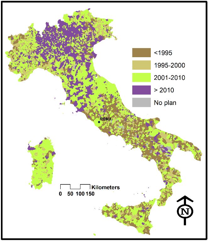
Land 2020, 9, 126                                                                                       6 of 12

GDPpc, and Ur), there is an important approach of the R2 coefficients to the maximum value with a
variation in the order of magnitude in comparison with the demographic ones (all close to or above 0.7)
with a geometry indisputably governed by the latitudinal gradient. The least contaminated parameter
in this sense is the level of university education (Udr) of the population aged between 30 and 34,
which fluctuates relatively little between regions (SD = 0.16) and is recorded by the trend curve in
fairly reliable form (R2 = 0.53); there is a slight predominance of the regions of Central Italy, but with
a distribution that is not particularly penalizing towards the south of the country. The PE does not
manifest itself in a striking form when considering the distribution of the areas of environmental value
(Par, N2kr, Fr): these areas, which are important because they host much of the national ecological
network [20], have fairly high SD values (above 0.4), which denote a high dispersion of conditions;
the R2 values remain very low (less than 0.08) and the latitudinal dependence appears so slight that
it cannot be considered statistically significant. The category with the greatest internal differences is
that of urban planning indicators, for which latitudinal sensitivity is often disjointed and therefore
dominated by more local dynamics. The SD values produce a scenario of behavioral independence,
at least for the Ud, Upc, and Uvr (urbanization variation rate) indicators (SD higher than 0.3), while
the LTs parameter appears less dispersed (SD = 0.04). The greater visibility of the latitudinal gradient
regards the Uvr parameter which, with an R2 = 0.35, shows a center–south which, in the last half
century, has seen its urbanized areas grow proportionately well more than the northern regions,
acquiring per capita urbanization levels (Upc) which are fully comparable and certified on the national
average of approximately 370 m2 /inhab. On the other hand, the other indicator of settlement behavior
(the first is precisely the Upc), or the LTs (land take speed), which shows a huge misalignment of the
regions even if a prevalence is distilled in a group of central and northern regions, is difficult to refer to
a homogeneous behavior.
      It is quite interesting to evaluate how aligned behaviors on the urban growth and higher
education front do not have equally aligned consequences on the economic and social front. Evidently,
the entrepreneurial advantages coming from the construction industry have not remained localized in
the center–south, where they have only produced negative environmental effects and temporary and
secondary economic returns.
      In summary, the functions that derive from the latitudinal processing of the 14 indicators analyzed
are aggregated into 4 clusters of types (Figure 4):
      1. a low PE on 2 environmental indicators (Fr and N2kr) and urban dynamics (DVR and LTs);
      2. a slight phenomenological prevalence in the central peninsula for three social indicators (Dd,
Ud, and OAI);
      3. a net incremental PE from north to south for an environmental indicator (Par), a social one (Ur),
and an urban one (Uvr);
      4. a net decreasing PE from north to south for two economic indicators (AI and GDPpc) and an
urban one (Upc).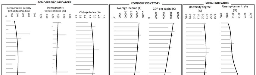
Land 2020, 9, 126                                                                                                                  7 of 12
     Land 2020, 9, x FOR PEER REVIEW                                                                                     2 of 12

                                                                (a).

                                                                (b).

      Figure  2. Indicators
          Figure  2. Indicatorsofoflatitude   sensibility.(a,b)In
                                    latitude sensibility.   (a,b)Inthethe   figures
                                                                        figures therethere  areplots
                                                                                      are the    the showing
                                                                                                      plots showing
                                                                                                              the trendthe
                                                                                                                         of trend
      of the
          theindicator
              indicator values    alongthe
                         values along      thelatitudinal
                                               latitudinal   axis
                                                          axis  of of
                                                                    thethe  peninsula
                                                                         peninsula  withwith   the maps
                                                                                          the maps         showing
                                                                                                      showing        the spatial
                                                                                                               the spatial
      distribution   by by
          distribution  region
                           regionofofthe
                                       thesame
                                            sameindicators    classifiedbybyrange.
                                                  indicators classified        range.
Land 2020, 9, 126 8 of 12
Land 2020, 9, x FOR PEER REVIEW 3 of 12
Land 2020, 9, x FOR PEER REVIEW 3 of 12
Figure3.3.Relationship
Figure Relationshipbetween
betweenstandard
standarddeviation
deviation(SD) andRR2 2parameters.
(SD)and parameters.
Figure 3. Relationship between standard deviation (SD) and R2 parameters.
Figure4.4. Peninsula
Figure Peninsulaeffect
effect(PE)
(PE)function
functioncluster.
cluster.
Figure 4. Peninsula effect (PE) function cluster.
3.2.
3.2.Comparative
ComparativeAssessment
Assessment
3.2. Comparative Assessment
Italy
Italyisisactually much
actually muchmoremore
uniform along the
uniform latitudinal
along axis than axis
the latitudinal the dominant
than theand widespread
dominant and
Italy
thought is actually
expresses; ormuch
at leastmore
it is uniform
in many along
importantthe latitudinal
aspects, such axis
as than the
environmental
widespread thought expresses; or at least it is in many important aspects, such as environmental dominant
quality and
and
widespread
quality andthought
biodiversity, expresses;
demographic
biodiversity, or at least
variations,
demographic it is in many
population
variations, important
structure,
population and aspects,
degree
structure, of
and such as environmental
education.
degree ofIn the face of
education. In
quality
these
the faceand biodiversity,
components, demographic
which are notwhich
of these components, variations,
extremely
are notvariablepopulation
between
extremely structure, and
the geographical
variable degree
between thepositions of education. In
of thepositions
geographical regions,
the
of face
there ofthe
theare these
regions, components,
social and
there are the which
economic
social are
andnot
ones, which extremely
economicshowones, variable
such between
a clear
which gradient
show theasageographical
such to positions
be indisputable
clear gradient [21]
as to be
ofwhich,
the regions, there
for the[21]
indisputable same are the
otherfor
which, social
resources, and economic
the sameisother
rather ones, which
contradictory.
resources, is rather show
Many such a
explanations
contradictory. clear
Many gradient as
thatexplanations to
are formulated be
that
indisputable
are formulated [21] in
which, for the same
the political other fields
and media resources,
applyistoo
rather contradictory.
simplistic equations, Manyoneexplanations that
of the most typical
are
offormulated in the to
which is linked political and media
the action fields apply
of organized crimetooinsimplistic
economicequations,
management one of theHowever,
[22]. most typical this
of which is linked to the action of organized crime in economic management [22]. However, thispeninsula, extended for about 900 km in the Mediterranean, is innervated by more than 600 km of
TAV (high-speed railway), 2000 km of inter-city railways, about 2500 km of motorways and 26
airports, of which at least 9 have multi-day communications with the regions of Northern Italy
(Figure 5).
Land 2020, 9, 126 9 of 12
The TAV railway lines arrive on the Tyrrhenian coast up to Salerno; that is, covering almost 4/5
of the peninsular development and more than half of the geographical area defined as Central and
Southern
in Italy, while
the political the opposite
and media Adriatic
fields apply toocoast, despite
simplistic not having
equations, onethe
of TAV line, typical
the most has been ofequipped
which is
linked to the action of organized crime in economic management [22]. However, this cannotseveral
with inter-city trains for many years, which ensure connections throughout the development be the
reason alone behind such an accentuated economic weakness; in recent decades, organized crime just
times a day. The exchanges of interest with the northern regions are continuous and intense: has
think ofwidely
spread summer tourism that
throughout the sees real exoduses
peninsula from the in
and in particular north to theareas.
its richer south Asforwas
seaside activities,
mentioned at
withbeginning
the a large spread
of thisofpaper,
seconda homes in allcause
reasonable the Tyrrhenian–Adriatic–Ionian
could lie in the length and coastal areasof
inefficiency and
themajor
land
and minor lines,
connection islands.
butThere
even is
thisnofactor
doubtcannot
that southern societyasmanifests
be so decisive, behavioral
it is true that mobilityinefficiencies
in the south in is
public–private management [24] and in territorial planning. The PE that
more difficult [23], but the entire peninsular length is affected by motorway lines, and thewe talked about in the article
transport
re-emerges
of goods byquite road categorically
is very intense inevery
the survey conducted the
day throughout on the
year.provision and updating
The peninsula, extendedof the
for urban
about
planning tools of the municipalities (Figure 6); but in truth with many
900 km in the Mediterranean, is innervated by more than 600 km of TAV (high-speed railway), 2000 km exceptions concerning
Sardinia,
of Sicily,
inter-city and Puglia
railways, aboutwhich
2500 km place them at a comparable
of motorways level with
and 26 airports, some
of which atnorthern regions,
least 9 have such
multi-day
as Friuli or Piedmont
communications with and Liguriaof[25],
the regions which Italy
Northern hardly anyone
(Figure 5). in Italy would say are lagging behind
on the side of their municipal planning.
Figure
Figure 5. Main infrastructural
5. Main infrastructural peninsula
peninsula equipment.
equipment.
The TAV railway lines arrive on the Tyrrhenian coast up to Salerno; that is, covering almost 4/5
of the peninsular development and more than half of the geographical area defined as Central and
Southern Italy, while the opposite Adriatic coast, despite not having the TAV line, has been equipped
with inter-city trains for many years, which ensure connections throughout the development several
times a day. The exchanges of interest with the northern regions are continuous and intense: just think
of summer tourism that sees real exoduses from the north to the south for seaside activities, with a
large spread of second homes in all the Tyrrhenian–Adriatic–Ionian coastal areas and major and minor
islands. There is no doubt that southern society manifests behavioral inefficiencies in public–private
management [24] and in territorial planning. The PE that we talked about in the article re-emerges
quite categorically in the survey conducted on the provision and updating of the urban planning
tools of the municipalities (Figure 6); but in truth with many exceptions concerning Sardinia, Sicily,
and Puglia which place them at a comparable level with some northern regions, such as Friuli or
Piedmont and Liguria [25], which hardly anyone in Italy would say are lagging behind on the side of
their municipal planning.Land 2020, 9, 126 10 of 12
Land 2020, 9, x FOR PEER REVIEW 5 of 12
Figure 6. Geographical
Figure 6. Geographical distribution
distribution of
of plan update thresholds
plan update thresholds (credit:
(credit: re-processing
re-processing of National
of National
Institute of Urban Planning-INU, 2016 data).
Institute of Urban Planning-INU, 2016 data).
4. Conclusions
4. Conclusions
The survey
The survey carried
carried outout and
and presented
presented in in the
the work
work is is aimed
aimed at at highlighting
highlighting thethe macroscopic
macroscopic
contradictions that the Italian peninsula manifests towards some socio-economic,
contradictions that the Italian peninsula manifests towards some socio-economic, environmental, and environmental,
and settlement
settlement phenomena
phenomena which,
which, in normal
in normal communication,
communication, aregenerally
are generallyexposed
exposed with
with excessive
excessive
simplification. Certainly,
simplification. Certainly, aa central
central aspect
aspect that
that then
then becomes
becomes aa driving
driving force
force for
for reflection
reflection for
for all
all the
the
others is the great energy of urban transformation that has affected this geographical area in the last
50 years, without significant differences with the continental national areas. Indeed, some indicators
such as the Uvr (urbanization variation rate) show an incremental curve markedly accentuated with
decreasing latitude (Figure 2). However, However, this this remarkable
remarkable construction
construction andand urban
urban planning
planning activity,
activity,
which has lasted for more than half a century at a speed speed completely
completely comparable with that of Northern
Italy, has
Italy, has failed to cause stable economic consequences.
consequences. Other analogies concern the alignment of the
country, aapeninsular
country, peninsular and continental
and continentalpart,part,
with with
respect to the seniority
respect of the population,
to the seniority the university
of the population, the
education rate,
university and the
education provision
rate, and theofprovision
naturalistic–environmental values, but all
of naturalistic–environmental this does
values, notthis
but all prevent
does
the economic
not prevent the andeconomic
employment andquality from being,
employment dramatically
quality from being,and with rigorous statistical
dramatically and with reliability,
rigorous
unbalanced
statistical towardsunbalanced
reliability, the south with progressive
towards the south latitudinal variation.
with progressive This work
latitudinal does not
variation. Thispretend
work
to provide answers to this complex condition of inconsistency, which, however,
does not pretend to provide answers to this complex condition of inconsistency, which, however, has worsened more
has
and more over
worsened morethe andyears,
moredespite
over thethe governments’
years, despite theattempts to compensate
governments’ attemptsand stem it [26,27],
to compensate andbutstemit
also
it wants
[26,27], buttoitpoint out, also
also wants usingout,
to point the also
other supporting
using the otherconsiderations (Figures 5 and
supporting considerations 6), how
(Figures it is
5 and
necessary
6), how it istonecessary
activate more incisive
to activate research
more andresearch
incisive intervention channels capable
and intervention of reading
channels capablephenomena
of reading
with different
phenomena optics
with from the
different past.from the past.
optics
Author Contributions:
Author Contributions: All All authors
authors have
have read
read and
and agree
agree toto the
the published
published version
version of
of the
the manuscript.
manuscript.
Conceptualization,
Conceptualization, B.R. and L.F.;
L.F.; methodology,
methodology, L.F.;
L.F.;data
datacuration,
curation,C.D.D.
C.D andand V.T.; writing—original draft
V.T.; writing—original
preparation,
preparation, B.R.
B.R. and
and L.F.;
L.F.; writing—review
writing—reviewand andediting,
editing,L.F.;
L.F.;supervision,
supervision,B.R.
B.R.
This research
Funding: This
Funding: research was
was funded
funded byby 2019
2019 RIA
RIA Project
Project (Research
(Research of
of L’Aquila
L’Aquila University
University Interest).
Interest).
Acknowledgments: We thank Prof. Alessandro Marucci and Prof. Francesco Zullo for suggestions and indications
Acknowledgments: We
relating to the retrieval thankused
of data Prof.
for Alessandro
research, andMarucci and Prof.
the anonymous Francesco
reviewers who,Zullo for suggestions
with their and
comments, have
indications
allowed us torelating to the improve
significantly retrieval the
of data used
quality for paper.
of the research, and the anonymous reviewers who, with their
comments, have allowed us to significantly improve the quality of the paper.
Conflicts of Interest: The authors declare no conflict of interest.
Conflicts of Interest: The authors declare no conflict of interest.Land 2020, 9, 126 11 of 12
References
1. Brown, J.W. The peninsular effect in Baja California: An entomological assessment. J. Biogeogr. 1987, 14,
359–365. [CrossRef]
2. Means, D.B.; Simberloff, D. The Peninsula Effect: Habitat-Correlated Species Decline in Florida’s
Herpetofauna. J. Biogeogr. 1987, 14, 551–568. [CrossRef]
3. Brown, J.W.; Opler, P.A. Patterns of Butterfly Species Density in Peninsular Florida. J. Biogeogr. 1990, 17,
615–622. [CrossRef]
4. Wiggins, D.A. The Peninsula Effect on Species Diversity: A Reassessment of the Avifauna of Baja California.
Ecography 1999, 22, 542–547. [CrossRef]
5. Jo, Y.S.; Stevens, R.D.; Baccus, J.T. Peninsula effect and species richness gradient in terrestrial mammals on
the Korean Peninsula and other peninsulas. Mammal Rev. 2017, 4, 266–276. [CrossRef]
6. Olivier, P.I.; Rolo, V.; Visser, N.; van Aarde, R.J. Correction: Pattern or process? Evaluating the peninsula
effect as a determinant of species richness in coastal dune forests. PLoS ONE 2018, 13, e0197623. [CrossRef]
[PubMed]
7. Whittaker, R.J.; Fernandez-Palacios, J.M. Island Biogeography: Ecology, Evolution, and Conservation; Oxford
University Press: Oxford, UK, 2007; p. 416. ISBN 0-19-856611-5.
8. Jenkins, D.G.; Rinne, D. Red herring or low illumination? The peninsula effect revisited. J. Biogeogr. 2008, 35,
2128–2137. [CrossRef]
9. Chubb, J. Patronage, Power and Poverty in Southern Italy: A Tale of Two Cities; Cambridge University Press:
Cambridge, UK, 1982; 292p.
10. Faini, R.; Galli, G.; Giannini, C. Finance and Development: The Case of Southern Italy. In Finance and
Development: Issues and Experience; Giovannini, A., Ed.; Cambridge University Pres: Cambridge, UK, 2001;
pp. 158–222.
11. Zamagni, V. The Economic History of Italy 1860-1990; Clarendon Press: Oxford, UK, 1993; 432p.
12. Romano, B.; Zullo, F.; Fiorini, L.; Marucci, A.; Ciabo, S. Land transformation of Italy due to half a century of
urbanisation. Land Use Policy 2017, 67, 387–400. [CrossRef]
13. Fiorini, L.; Zullo, F.; Marucci, A. Romano, B. Land take and landscape loss: Effect of uncontrolled urbanization
in Southern Italy. J. Urban Manag. 2018, 8, 42–56. [CrossRef]
14. ISPRA. Consumo di Suolo, Dinamiche Territoriali e Servizi Ecosistemici; Rapporto 2018; ISPRA: Roma, Italy,
2018; 280p.
15. Gascon, F.; Cadau, E.; Colin, O.; Hoersch, B.; Isola, C.; López Fernández, B.; Martimort, P. Copernicus
Sentinel-2 Mission: Products, Algorithms and Cal/Val. In Proceedings of the SPIE 2018, 9218, Earth Observing
Systems XIX, 92181E, San Diego, CA, USA, 26 September 2014. [CrossRef]
16. Geudtner, D.; Torres, R.; Snoeij, P.; Davidson, M.; Rommen, B. Sentinel-1 System Capabilities and Applications.
In Proceedings of the 2014 IEEE Geoscience and Remote Sensing Symposium, Quebec city, QC, Canada,
13–18 July 2014. [CrossRef]
17. Stathakis, D.; Tsilimigkas, G. “Measuring the compactness of European medium-sized cities by spatial
metrics based on fused data sets”. Int. J. Image Data Fusion 2014, 6, 42–64. [CrossRef]
18. Chorianopoulos, I.; Pagonis, T.; Koukoulas, S.; Drymoniti, S. Planning, competitiveness and sprawl in the
Mediterranean city: The case of Athens. Cities 2010, 27, 249–259. [CrossRef]
19. Lagarias, A.; Sayas, J. Urban sprawl in the mediterranean: Evidence from coastal medium-sized cities.
Reg. Sci. Inquiry 2018, 10, 15–32.
20. Filpa, A.; Romano, B. (Eds.) Pianificazione e reti Ecologiche, Planeco; Gangemi, Ed.: Roma, Italy, 2003;
ISBN 88-492-0487-6.
21. Coccia, M. A New Approach for Measuring and Analysing Patterns of Regional Economic Growth: Empirical
Analysis in Italy. Sci. Reg. 2009, 8, 71–95. [CrossRef]
22. Pinotti, P. Organized Crime, Violence, and the Quality of Politicians: Evidence from Southern Italy. In Lesson
from the Economics of Crime; Cook, P.J., Machin, S., Marie, O., Mastrobuoni, G., Eds.; MIT Press: Cambridge,
MA, USA, 2013; pp. 175–188.
23. Giorgio, S.; Benedetto, T. A Territorial Analysis of Infrastructures in Italy. In Proceedings of the 42nd Congress
of the European Regional Science Association: “From Industry to Advanced Services—Perspectives of
European Metropolitan Regions”, Dortmund, Germany, 27–31 August 2002.Land 2020, 9, 126 12 of 12
24. Antellini Russo, F.; Zampino, R. Infrastructures, Public Accounts and Public-Private Partnerships: Evidence
from the Italian Local Administrations. Rev. Econ. Inst. 2012, 3, 1–28. [CrossRef]
25. Romano, B.; Zullo, F.; Marucci, A.; Fiorini, L. Vintage Urban Planning in Italy: Land Management with the
Tools of the Mid-Twentieth Century. Sustainability 2018, 10, 4125. [CrossRef]
26. Paini, A. Italy’s ‘Southern Question’: Orientalism in One Country. Australian J. Anthropol. 2001, 12, 415–417.
27. Rosengarten, F. The contemporary relevance of Gramsci’s views on Italy’s “Southern question”. In Perspectives
on Gramsci, Politics, Culture and Social Theory; Routledge: Abingdon-on-Thames, UK, 2009. [CrossRef]
© 2020 by the authors. Licensee MDPI, Basel, Switzerland. This article is an open access
article distributed under the terms and conditions of the Creative Commons Attribution
(CC BY) license (http://creativecommons.org/licenses/by/4.0/).You can also read