Learning to Swarm with Knowledge-Based Neural Ordinary Differential Equations - arXiv
←
→
Page content transcription
If your browser does not render page correctly, please read the page content below
Learning to Swarm with Knowledge-Based Neural Ordinary
                                                                    Differential Equations
                                                                               Tom Z. Jiahao∗ , Lishuo Pan∗ and M. Ani Hsieh

                                            Abstract— Understanding single-agent dynamics from collec-        a top-down approach to controller synthesis. Various data-
                                         tive behaviors in natural swarms is crucial for informing robot      driven methods have been used to model local control policy
                                         controller designs in artificial swarms and multiagent robotic       in swarms. Feedforward neural networks have been used
                                         systems. However, the complexity in agent-to-agent interactions
                                         and the decentralized nature of most swarms pose a significant       to approximate decentralized control policies by training
                                                                                                              on the observation-action data from a global planner [14].
arXiv:2109.04927v2 [cs.RO] 13 Sep 2021

                                         challenge to the extraction of single-robot control laws from
                                         global behavior. In this work, we consider the important task        Furthermore, deep neural networks have been used to model
                                         of learning decentralized single-robot controllers based solely on   higher order residual dynamics to achieve stable control in a
                                         the state observations of a swarm’s trajectory. We present a gen-    swarm of quadrotors [17]. Recently, graph neural networks
                                         eral framework by adopting knowledge-based neural ordinary
                                         differential equations (KNODE) – a hybrid machine learning           (GNN) have been extensively used in swarms, owing to
                                         method capable of combining artificial neural networks with          their naturally distributed architecture. GNN allows efficient
                                         known agent dynamics. Our approach distinguishes itself from         information propagration through networks with underlying
                                         most prior works in that we do not require action data for           graphical structures [22], and have been noted for their sta-
                                         learning. We apply our framework to two different flocking           bility and permutation equivariance [4]. Decentralized GNN
                                         swarms in 2D and 3D respectively, and demonstrate efficient
                                         training by leveraging the graphical structure of the swarms’        controllers have been trained with global control policies to
                                         information network. We further show that the learnt single-         imitate flocking [22]. All these works poses the controller
                                         robot controllers can not only reproduce flocking behavior in        synthesis problem as an imitation learning problem, and
                                         the original swarm but also scale to swarms with more robots.        require knowledge of the actions resulting from an optimal
                                                                                                              control policy for learning or improving the local controllers.
                                                               I. I NTRODUCTION                               In practice, action data can be difficult to access, especially
                                                                                                              when learning behaviors from natural or adversarial swarms.
                                            Many natural swarms exhibit mesmerizing collective be-            In addition, GNNs can potentially allow a robot to access the
                                         haviors [12], [3], [25], [1], and have fascinated researchers        state information of robots outside its communication range
                                         over the past decade [23]. A central question is how do these        through information propagation. The extent of decentraliza-
                                         behaviors emerge from local interactions. Such fascination           tion may therefore be limited when more propagation hops
                                         has led to much developments in artificial swarms and multi-         are allowed.
                                         agent robotic systems to emulate the swarms in nature. [13],            Deep reinforcement learning has also been applied to
                                         [20], [15].                                                          swarms for various applications [7]. Early works like [8]
                                            Some of the earliest works on developing swarm con-               learn a decentralized control policy for maintaining distances
                                         trollers rely heavily on physical intuitions and design con-         within a swarm and target tracking. An inverse reinforcement
                                         trollers in a bottom-up fashion. Boids was developed by              learning algorithm was presented in [18] to train a decen-
                                         combining rules of cohesion, alignment, and separation to            tralized policy by updating the reward function alongside
                                         mimic the flocking behavior in natural swarms [13]. [24]             the control policy based on an expert policy. In addition,
                                         proposed self-driven particles to investigate the emergence of       GNNs have also been used within the reinforcement learning
                                         collective behaviors in biologically motivated swarms. [20],         framework for learning connectivity for data distribution
                                         [19] designed flocking controllers for fixed and dynamic             [21]. However, reinforcement learning is usually employed
                                         network topologies with stability guarantees. These early            to solve task-specific problems with well-defined goals. The
                                         works laid the foundation of decentralized swarm control and         specific objectives of swarms may be difficult to discern from
                                         offered a glimpse of the myriad of possible swarm behaviors          only observations, and therefore reinforcement learning is
                                         achievable using local controllers.                                  often not suitable for learning single-agent control strategies
                                            Related Works Modern machine learning has enabled                 from solely observational data.
                                         pattern discovery from complex and high-dimensional data                The contribution of this work is three-fold. First, we
                                         sets. It opens up avenues for learning swarm controllers             demonstrate the feasibility of learning single-robot con-
                                         directly from observations of the swarm itself, providing            trollers that can achieve the observed global swarming be-
                                            This work was supported by ARL DCIST CRA W911NF-17-2-0181 and     haviors from only swarm trajectory data. Second, we propose
                                         Office of Naval Research (ONR) Award No. 14-19-1-2253.               a generalized model for incorporating known robot dynamics
                                            All authors in this work are with the GRASP Laboratory, Univer-   to facilitate learning single-robot controllers. Lastly, we show
                                         sity of Pennsylvania, Philadelphia, PA 19104, USA. {panls, zjh,
                                         m.hsieh}@seas.upenn.edu                                              how to efficiently scale KNODE for learning from local
                                            ∗ Equal contribution.                                             information in a multi-agent setting.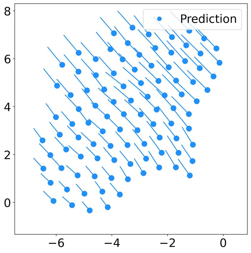
II. P ROBLEM F ORMULATION III. K NOWLEDGE - BASED N EURAL O RDINARY
D IFFERENTIAL E QUATIONS (KNODE)
We consider the problem of learning single-robot con-
KNODE is a scientific machine learning framework that
trollers based on the observations of the trajectory of a
applies to a general class of dynamical systems. It has been
swarm. We assume that the swarm is homogeneous, i.e.,
shown to model a wide variety of systems with nonlinear
all robots in the swarm use the same controller. Given a
and chaotic dynamics. In our problem, we assume a single-
swarm of n agents, we make m observations at sampling
robot dynamics in the form of (4). From a dynamical systems
times T = {t1 , t2 , ..., tm }, ti ∈ R given by
perspective, f (zi , ûθ ) is a vector field. This makes KNODE
T
Z (t1 )
z1 (t1 ) z2 (t1 ) · · · zn (t1 )
a suitable method for our problem because it directly models
ZT (t2 ) z1 (t2 ) z2 (t2 ) · · · zn (t2 ) vector fields using neural networks [9]. To put KNODE in the
.. =
.. .. .. .. ,
context of our learning problem, given some known swarm
. . . . . dynamics f˜(Z) as knowledge, KNODE optimizes for the
ZT (tm ) z1 (tm ) z2 (tm ) · · · zn (tm ) control law as part of a dynamics given by
żi (t) = fˆ(zi , ûθ , f˜(Z)), (5)
where the matrix Z(ti ) ∈ Rn×d is the observations of the
states of all n agents at ti , and the vector zi (tj ) ∈ Rd is where the control law ûθ is a neural network, and fˆ defines
the state of agent i observed at tj with dimension d. For the coupling between the knowledge and the rest of the dy-
instance, in a first-order system, an agent modeled as a rigid namics. While the original KNODE linearly couples a neural
body in a 3-dimensional space has d = 6, where the first network with f˜ using a trainable matrix Mout [9], we note
three dimensions correspond to the positions and the last that the way knowledge gets incorporated is flexible. In later
three the orientations. Our goal is to learn a single-robot sections we will demonstrate how to effectively incorporate
controller solely from the observations Z. knowledge for learning single-robot controllers. Furthermore,
The evolution of each individual robot’s state can be the ability to incorporate knowledge will require less training
described by the true dynamics given by data [10], [9].
We minimize the mean squared error (MSE) between the
żi (t) = fi (zi , ui ), (1) observed trajectories and the trajectories predicted from the
estimate dynamics using ûθ for robot i. A loss function is
where zi is the state of robot i, and ui is its control law. given by
The function fi (·, ·) defines the dynamics given the state m−1 n
1 XX
of robot and control law ui . It is assumed that all robots L(θ) = kẑi (tj+1 , zi (tj )) − zi (tj+1 )k2 , (6)
in the swarm have the same dynamics and control strategy, m − 1 j=1 i=1
and therefore we can drop the subscripts and rewrite (1) as where ẑi (tj+1 , zi (tj )) is the estimated state of robot i at
żi (t) = f (zi , u) for all i. The control law u is a function tj+1 generated using the initial condition zi (tj ) at tj , and
of the states of other robots in the swarm, and defines the it’s given by
interaction between robot i. For example, a control law u can Z tj+1
be designed to let each robot only interact with its neighbors ẑi (tj+1 , zi (tj )) = zi (tj ) + fˆ(zi , ûθ , f˜(Z))dt. (7)
within some communication radius. tj
The dynamics of the entire swarm can be written as a Intuitively, the loss function in (6) computes the one-step-
collection of the single-robot dynamics as ahead estimated state of all robots from every snapshot in
the observed trajectory, and then computes the average MSE
Ż(t) = [ż1 (t), ż2 (t), · · · , żn (t)]T . (2) between the estimated and observed states for the entire
trajectory form t1 to tm−1 .
Given the initial conditions of all robots Z0 at t0 , the states Our learning task can then be formulated as an optimiza-
of all robots at t1 is given by tion problem given by
Z t1 min L(θ), (8)
Z(t1 ) = Z0 + Ż(t)dt. (3) θ
t0 s.t. żi = fˆ(zi , ûθ , f˜(Z)), for all i, (9)
In practice, the integration in (3) is performed numerically. which includes the dynamics constraint for all robots in
Our task is to find a single-robot control law parameterized the swarm. The parameters θ can then be estimated by
by θ as part of the single-robot dynamics given by θ = arg minθ L(θ). The gradients of θ with respect to
the loss can be computed by either the conventional back-
żi (t) = fˆ(zi , ûθ ), (4) propagation or the adjoint senesitivity method. The adjoint
sensitivity method has been noted as a more memory efficient
where ûθ is the single-robot control law parameterized by approach than backpropagation, though at the cost of training
θ. The learnt controller should best reproduce the observed speed [5]. In this work, we use the adjoint method for training
swarm behaviors. similar to that in [2] and [9].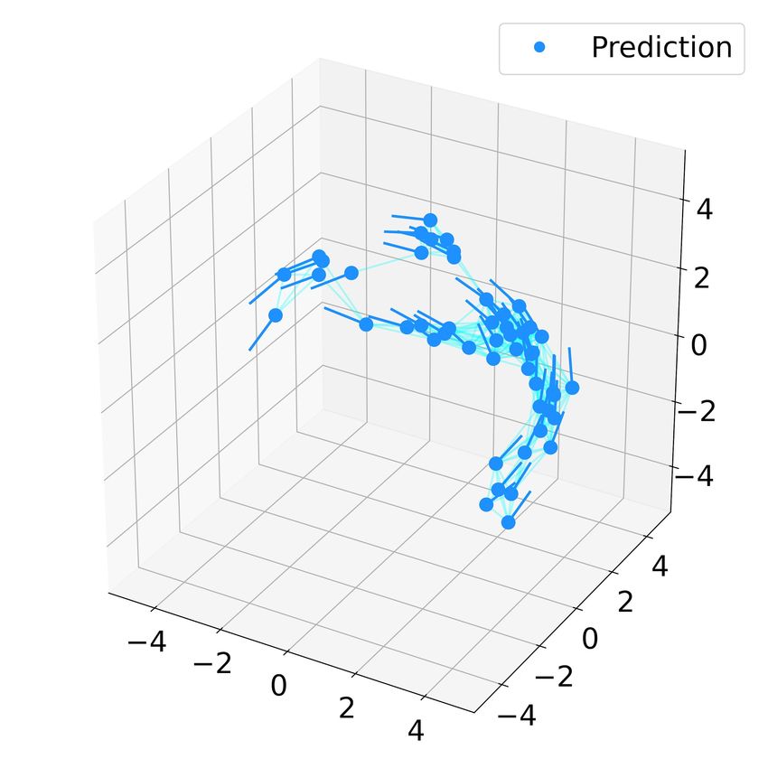
IV. M ETHOD
   In this section, we walk through the process to construct
fˆ(zi , ûθ ) in the context of learning to swarm and the                                     1
incorporation of knowledge in the form of known single                           dcr
                                                                                          0       2
robot dynamics.

A. Decentralized Information Network                                                              3

   We assume a robot in a swarm can only use its local
information as inputs to its controller. To incorporate this
assumption, we impose a decentralized information network          Fig. 1. Decentralized information network for robot 0 with time delay τ ,
on the swarm. Specifically, we assume robots have finite           and 3 active neighbors. The image shows robot 0’s egocentric view, where
communication ranges and can only communicate with a               8 neighbors are within its communication range dcr . Only the closest three
                                                                   neighbors contribute to the information structure of robot 0. Their states
fixed number of neighbors, denoted by k, within this range.        from t − τ are ordered based on their proximity to robot 0 to form Y0 (t).
We denote the communication radius by dcr . We refer to
these neighbors as the active neighbors. If there are more
than k neighbors within a robot’s communication radius, only       real swarms. With time delay, the information structure of
the closest k neighbors are considered to be the active ones.      robot i in (11) becomes
   We leverage the communication graph of the swarm to
compute the local information for each robot at each time              Yi (t) = g({zj (t − τ )|i 6= j, j ∈ Ni (t − τ )}, k).            (12)
step. The communication graph at time t can be described              Fig. 1 shows an example of the information structure
by a graph shift operator S(t) ∈ Rn×n , which is a binary          described by (12) using k = 3. The process of constructing
adjacency matrix computed based on dcr and the positions           Yi (t) for all t ∈ T in (10), (11) and (12) leverages
of all robots at each time step. In this work, we treat            the graphical structure of the swarm’s information network.
the communication radius dcr as a hyperparameter. Note             During training, the collection of delayed neighbor infor-
that the communication graph is time-varying because the           mation is done efficiently through the matrix multiplication
information network changes as robots move around in a             S(t − τ )Z(t − τ ), which leaves for each robot only the
swarm. Then Sij (t) = 1 if the Euclidean distance between          state information of its neighbors at t − τ . Then for robot
agents i and j is less than or equal to dcr , and Sij (t) = 0      i we append the ith row of [S(t − τ )Z(t − τ )] to its own
otherwise. The index set of the neighbors of robot i at time       state zi (t). Finally we only keep k rows of the resulting
t is therefore given by                                            matrix to form Yi (t). Compared to some GNN approaches
               Ni (t) = {j|j ∈ I, Sij (t) = 1},            (10)    [22], [4], the information structure Yi (t) in our work is
                                                                   more explicit. A robot with GNN controllers can only access
where I = 1, . . . , n is the index set of all robots. Note that   the diffused state information from other robots, i.e. the
set of neighbors of robot i also includes itself. At time t,       neighbors’ information has been repeatedly multiplied by
the information kept by robot i is the matrix Yi (t) ∈ Rk×d        the graph operators before reaching this robot. In this work,
given by                                                           we directly let each robot access the state information of
                                                                   its active neighbors. In real-world implementation of robot
              Yi (t) = g({zj (t)|j ∈ Ni (t)}, k),          (11)    swarms, our proposed information structure in (12) is more
where the function g(·, k) maintains the dimension of the          realistic as each robot can easily subscribe to or observe
matrix Yi (t), and forms the rows of matrix Yi (t) using the       its neighbors’ states. In addition, the information structure
state information of robot i’s active neighbors in descending      Yi (t) enables scalable learning as we can treat the robots
order of their Euclidean distance from robot i. If there are       in a swarm as batches. As a result, training memory scales
fewer than k active neighbors within a robot’s communica-          linearly with the number of robots in the swarm, and training
tion radius, the remaining rows in Yi (t) are padded with          speed scales sub-linearly.
zeros. In this work, k is treated as a hyperparameter.             C. Knowledge Embedding
   The matrix Y(t) represents the local information accessi-
                                                                      In this work, a potential-function-based obstacle avoidance
ble to each robot at time t and it completes the decentralized
                                                                   strategy similar to [11] is used as knowledge. Let the distance
information network of the swarm. In summary, (10) and
                                                                   between robot i and an obstacle O be dO (zi ), where zi is
(11) enforces the assumptions of finite communication and
                                                                   the state and includes the position of robot i. The potential
perception radii for each robot.
                                                                   function is then given by
B. Information Time Delay                                                                 (
                                                                                             λ    1
                                                                                                2       if dO (zi ) ≤ d0 ,
   In addition to a decentralized information structure, we                    UO (zi ) = 2 dO (zi )                          (13)
                                                                                            0           otherwise,
further assume that each robot only gets delayed state
information from its neighboring robots by a time lag τ .          where λ is the gain, and d0 is the obstacle influence threshold
This is to emulate the latency in agent communication in           (i.e. the distance within which the potential function becomes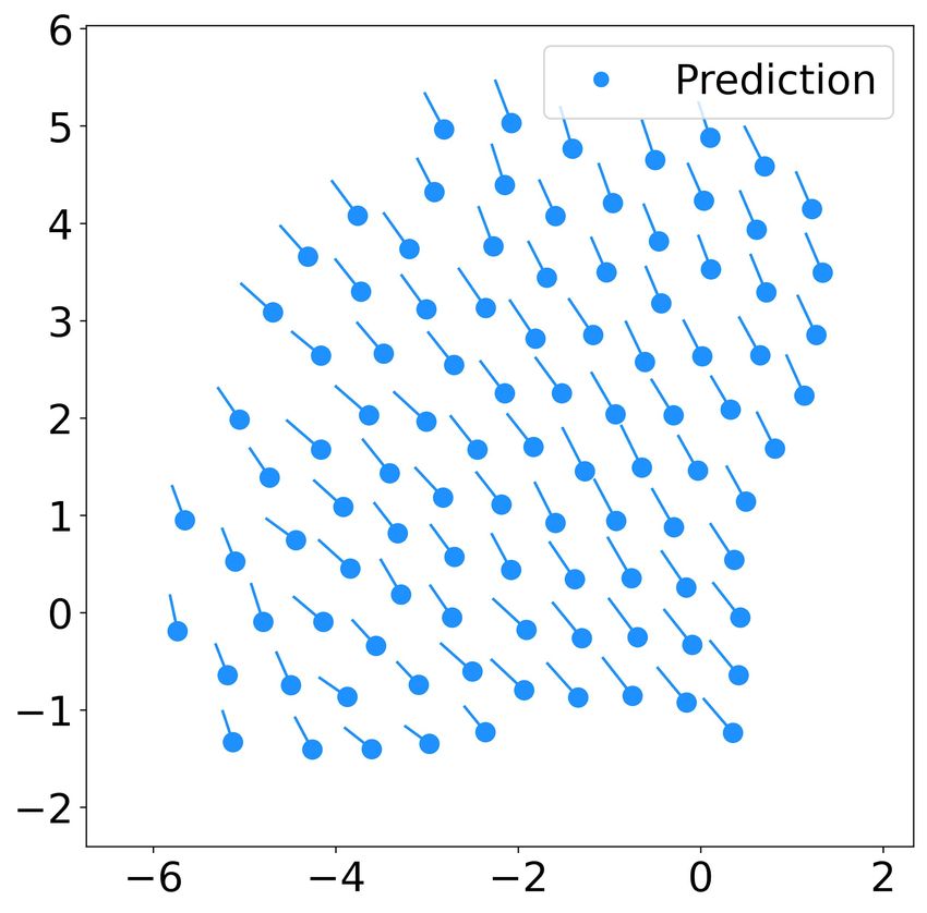
active). Based on this potential function, the repulsive force      The lengths of the trajectories is chosen such that the swarms
to avoid the obstacle O is given by                                 will converge to stable flocking. We use 30 trajectories as the
                     (                                              training data, and the remaining 5 as the testing data. We
                       −∇UO (zi ) if dO (zi ) ≤ d0 ,                added zero-mean Gaussian noise with variance 0.001 to the
          FO (zi ) =                                      (14)
                       0            otherwise,                      training trajectories. This is known as stabilization noise in
                                                                    modeling dynamical systems and has been shown to improve
   When multiple obstacles are present, the repulsive forces
                                                                    model convergence [26].
computed from each obstacle are summed for a resultant
                                                                       The training model follows (15). There are no obstacles
repulsive force. For collision avoidance, we assume that each
                                                                    to avoid in the 2D case, so the potential function is only
agent will only actively avoid its closest neighbor within d0
                                                                    used to avoid collision among the agents. Specifically, we
at any given time.
                                                                    let each robot avoid its closest neighbor at every time step.
   Assuming that the robots in a swarm follow first-order dy-
                                                                    For the controller ûθ , we use a one layer neural network
namics, we combine the decentralized information network
                                                                    with 128 hidden units, and a hyperbolic tangent activation
in (11) and the knowledge in (14) into a dynamics given by
                                                                    function. The trainable gain for collision avoidance is defined
                                         X                          as λ = a + φ2 , where a is a positive number for setting
         żi = fˆ(zi , ûθ (Yi , zi )) −   λj ∇UOj (zi ), (15)
                                                                    the minimum amount of force to avoid collision. The single
                                      j
                                                                    parameter φ is trained together with the neural network to
where uθ is a neural network, and λj is a trainable gain            provide more forces for collision avoidance as needed. We
for avoiding obstacle Oj . Both uθ and λj are trained using         do not assume information delay in the 2D case.
the KNODE framework. Note that since all robots in a
homogeneous swarm share the same control law, the training          B. Evaluating flocking in 2D
is done in batches of robots to accelerate training.                  We evaluate flocking behavior using two metrics:
              V. L EARNING TO FLOCK IN 2D                           Average velocity difference (avd) measures how well the
                                                                    velocities of robots are aligned in 2D flocking. It is given by
  We use a global controller proposed by [20] to generate
observations for our learning problem.                                                     2     X
                                                                             avd(t) =              ||vi (t) − vj (t)||2 .     (18)
A. Simulation in 2D and training                                                        n(n − 1)
                                                                                                   i6=j

  This global controller achieves stable flocking, which            Average minimum distance to a neighbor (amd) measures
ensures eventual velocity alignment, collision avoidance and        the cohesion between agents in both 2D and 3D when
group cohesion in a swarm of robots. The robots follow the          flocking is achieved. It is given by
double integrator dynamics given by
                                                                                              n
                                                                                          1X
                    ṙi = vi ,                                                 amd(t) =        min ||ri (t) − rj (t)||2 .     (19)
                                                            (16)                          n i=1 j
                    v̇i = ui , i = 1, ..., n,
where ri is the 2D position vector of robot i, vi is its velocity   amd should decrease as the robots move closer together, but
vector. The full state of each robot is therefore x = [r, v] ∈      it should not reach zero if collision avoidance is in place.
R4 . The control law ui is given by
                     X                 X                            C. 2D Results
           ui = −        (vi − vj ) −      ∇ri Vij ,         (17)      Fig. 2 shows 4 snapshots of one swarm trajectory gener-
                    j∈Ni                  j∈Ni
                                                                    ated using the trained single-robot controller. The communi-
where Vij is a differentiable, nonnegative, and radially            cation radius is 5 and the number of active neighbors is 6.
unbounded function of the distance between robot i and              The robots in the snapshots are initialized using the initial
j [20]. The first summation term in (17) aims to align              states from one of the testing trajectories. It can be observed
the velocity vector of robot i with those of its flockmates,        that at around t = 600, the predicted robots have mostly
while the second summation term is the total potential field        aligned their velocities in the same direction, indicating the
around robot i responsible for both collision avoidance and         emergence of flocking behavior. This can be further verified
cohesion [20]. The set Ni is the set of all robots in the swarm     by the metrics for 2D flocking as shown in Fig. 3. The
for the global controller.                                          predicted swarm follow similar trends as the ground truth
   We use the 4th order Runge-Kutta method to simulate the          under both metrics. Furthermore, we deployed the trained
dynamics in (17) with a step size of 0.01. The locations√of         controller on a larger swarm with 100 agents. Fig. 4 shows
robots are initialized uniformly on a disk with radius n            that the learnt controller generalizes to swarms with more
to normalize the density within the swarm. The velocities           agents and flocking emerges after about 800 steps. We do
of robots are initialized uniformly with magnitudes between         note that with some initialization, the 100-agent swarm tends
[0, 3]. Additionally, a uniformly sampled velocity bias with        to split into subswarms. This is not unexpected since stability
magnitude between [0, 3] is added to the swarm. A total of          of the original controller is only guaranteed under certain
35 trajectories are simulated, each with a total of 2000 steps.     conditions [20], [19].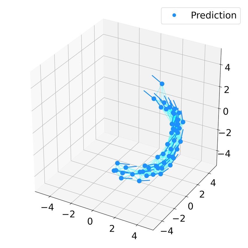
VI. L EARNING TO F LOCK IN 3D
(a) t=0 (b) t=100 Next, we apply our learning method on the 3D simula-
tion of boids. Boids were introduced to emulate flocking
behaviors and led to the creation of artificial life in the
field of computer graphics [13]. The flocking behavior of
boids is more challenging to learn because their steady state
flocking behavior is more complex than the 2D flocking
in the previous section when the swarm is confined within
limited volume.
(c) t=600 (d) t=1200
A. Simulation in 3D and training
Boids are simulated based on three rules:
• cohesion each boid moves towards the average position
of its neighboring boids.
• alignment each boid steer towards the average heading
of its neighboring boids.
• separation each boid steer towards direction with no
Fig. 2. Predicted trajectory of 10 robots using the learnt controller (dcr = obstacles to avoid colliding into its neighboring boids.
5, k = 6) with the same initial states as the testing data. The subfigures
(a)(b)(c)(d) show the snapshots of the swarm at t = 0, 100, 600, and 1200 While cohesion and collision avoidance are grouped into one
respectively. term in the 2D flocking case, boids use two separate terms.
Furthermore, the boids in simulation are confined in a cubic
space and are tasked to avoid the boundaries.
Boids are simulated in Unity [16]. We follow the default
settings with a minimum boids speed of 2.0, a maximum
(a) (b)
speed of 5.0, a communication range of 2.5, a collision
avoidance range of 1.0, a maximum steering force of 3.0, and
the weights of cohesion, alignment, and separation steering
force are all set to 1.0. For obstacle avoidance we set the
scout sphere radius as 0.27, the maximum search distance
as 5.0, and the weight of obstacle avoidance steering force
as 10.0. Boids are simulated in a cubic space with an equal
side length of 10, with each axis ranging from −5 to 5. The
Fig. 3. The metrics for the learnt 2D controller (dcr = 5, k = 6) show (a) boids’ positions are randomly initialized within a sphere of
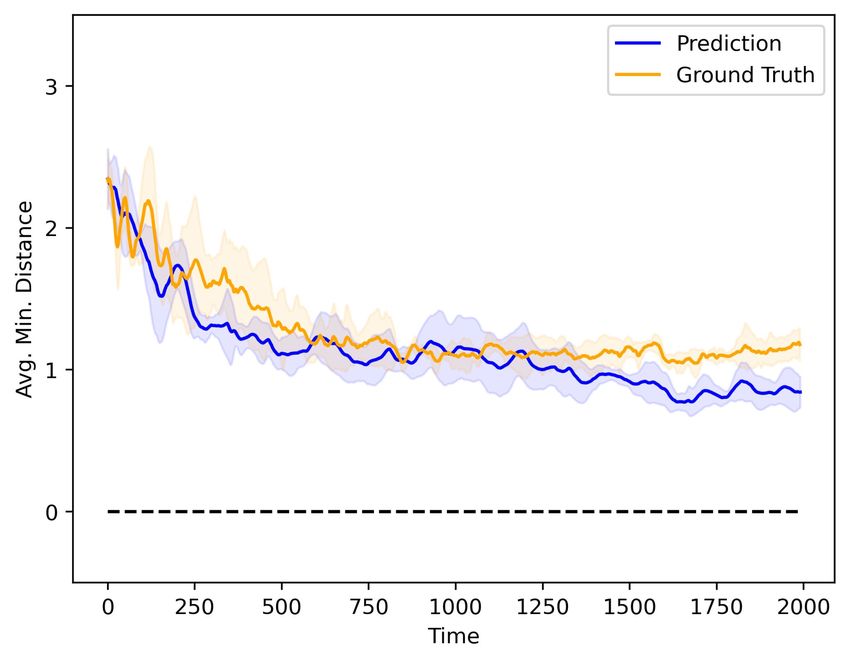
average velocity difference, and (b) average minimum distance to a neighbor.
The 95% confidence intervals are based on 5 sets of testing trajectories.
radius 5 centered at origin, and their velocities vectors are
randomly initialized with a constant magnitude.
Unity can log both the positions and velocities of boids.
However, to make the learning task more challenging, we
(a) (b) (c)
normalize the velocities before including them in the training
data, i.e., only the positions and orientation of the boids are
given. For a swarm of 10 boids we simulate 6 trajectories,
each with a total of 1700 steps. We discard the first 10 time
steps to remove simulation artifacts (There are ’jumps’ in the
first few steps of simulation) and only use the remaining 1690
steps. We use 2 trajectories for training and the remaining 4
(d) (e) (f)
as the testing data. Zero-mean Gaussian noise with variance
0.01 is added to the training trajectories.
The training model follows (15). The controller ûθ uses
a one layer neural network with 128 hidden units and a
hyperbolic tangent activation function. In addition to colli-
sion avoidance, we also avoid the boundaries of the cubic
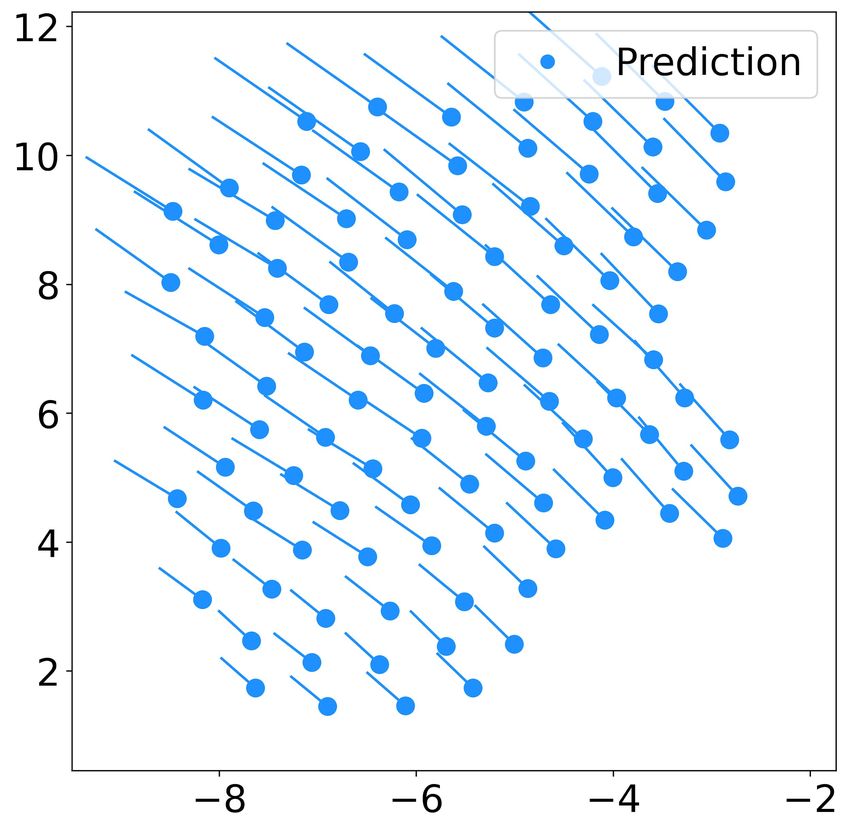
Fig. 4. Predicted trajectory of 100 robots using the learnt controller
space. This is implemented by avoiding the closest three
(dcr = 5, k = 6) with uniformly initialized positions and zero velocities. points on the boundaries in the three axes at any given time.
The subfigures (a)(b)(c)(d)(e)(f) show the snapshots of the swarm at t = Collision and obstacle avoidance use different trained gains,
0, 200, 400, 800, 1000 and 1200 respectively.
both of which are defined as λ = φ2 . We further assume an
information delay of 1.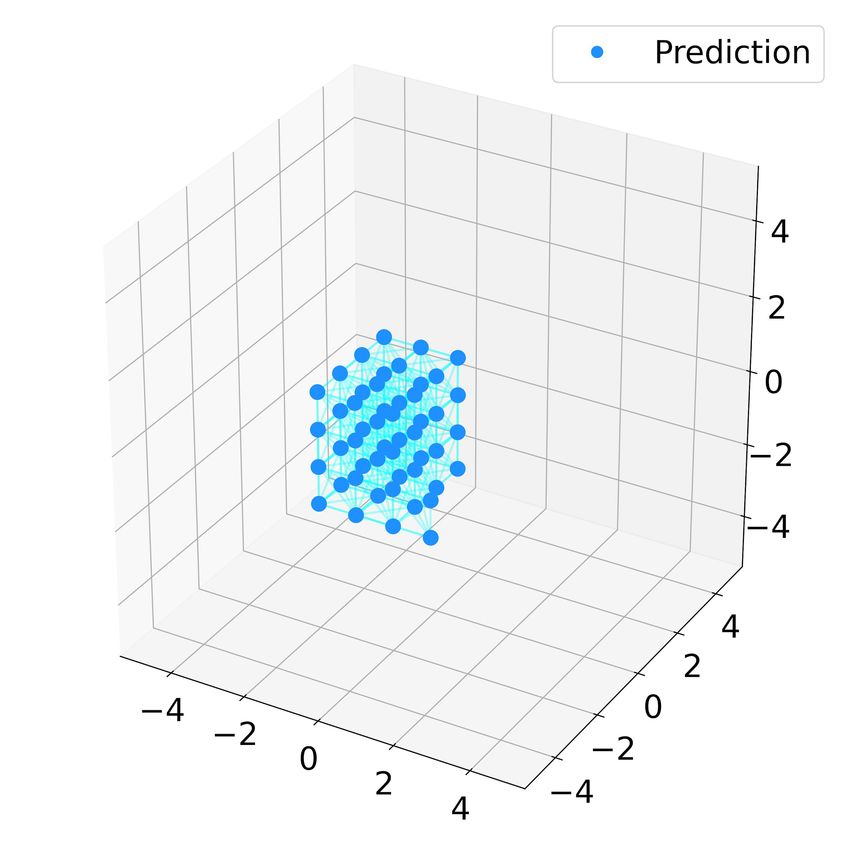
(a)                                 (b)
     (a.i)                  (a.ii)                   (a.iii)
     t=0                    t = 400                  t = 800

     (b.i)                   (b.ii)                  (b.iii)
     t=0                     t = 400                 t = 800

                                                                                Fig. 6. The metrics for the learnt 3D controller (dcr = 2, k = 6). (a)
                                                                                Average velocity difference in the predicted trajectory converges, and (b)
                                                                                the distribution of the first 10 POD modes of the predictions and ground
                                                                                truth are similar. The 95% confidence intervals are based on 4 sets of testing
                                                                                trajectories.

Fig. 5. Ground truth and predicted trajectories of 10 robots using the learnt
                                                                                     (a)                      (b)                     (c)
controller (dcr = 2, k = 6). The subfigures (a.i)(a.ii)(a.iii) show snapshots        t=0                      t=400                   t=600
of the ground truth trajectory at t = 0, 400, 800, and (b.i)(b.ii)(b.iii)
show the eventual flocking and the formation process of subswarms at
t = 0, 400, 800. The light blue lines connect the neighbors in the swarm.

B. Evaluating flocking in 3D
                                                                                Fig. 7. The flocking of 50 robots using the learnt controller (dcr = 2, k =
   Average minimum distance to a neighbor from (19) is                          6) with uniformly initialized positions and zero velocities. The subfigures
also used for 3D flocking to measure the cohesion between                       (a)(b)(c) show the snapshots of the swarm at t = 0, 400, 600 respectively.
robots. However, average velocity difference is not a good                      The light blue lines connect the neighbors in the swarm.
metric for evaluating flocking in 3D for two reasons: (1)
boids only align their velocity with the local flockmates
because of the presence of obstacles, and (2) boids form                                                  VII. D ISCUSSION
subswarms. As a result, velocity alignment is often not                            Our experiments show that the model proposed in (15) is
achievable at steady state flocking in boids. We instead com-                   able to learn flocking in both 2D and 3D. We treated the com-
pare the Proper orthogonal decomposition (POD) modes                            munication radius dcr and the number of active neighbors k
of the true and predicted trajectory to check how similar the                   as hyperparameters that need to be tuned during training. The
energy distributions are in their respective dynamics. POD                      choices of dcr and k and the corresponding learnt controllers
is a model order reduction technique which decomposes the                       can inform how the extent of decentralization can affect
trajectory of a system into modes based on their energy                         flocking behavior in robot swarms. We perform a grid search
[6]. Systems with similar dynamics should have similar                          using different dcr and k for 2D flocking. To evaluate the
distributions of POD modes.                                                     performance of flocking in 2D in the grid search, we use a
                                                                                single number metric, namely the velocity variance which is
                                                                                given by
C. 3D Results                                                                                                        " n          # 2
                                                                                                m n
                                                                                            1 XX                   1 X
   Fig. 5 shows the testing data and the swarm trajectories                           C=                vj (ti ) −       vk (ti )     .   (20)
                                                                                            n i=1 j=1              n
generated using the learnt controller. It uses a communica-                                                                    k=1

tion radius of 2 and the number of active neighbors is 6.                          This metric measures the spread of robot velocities
The robots are initialized using the same initial states as                     throughout time. It should be small if robots reach concensus
the testing trajectory. The predicted trajectories shows the                    in their velocities. Fig. 8 shows the grid search result. We
formation of subswarms during steady state flocking similar                     observe that for small proximity radii or small number of
to that of the testing trajectory. Note that when the robots are                active neighbors, the velocity variance tends to be large. This
initialized closer to each other, they are more likely to form a                matches our intuition as a small dcr or k means that each
single swarm during steady state flocking. The metrics for the                  robot can communicate with fewer neighbors and therefore
learnt controller are shown in Fig. 6. It can be seen that group                has less information to act upon in order to stay connected
cohesion is achieved as both the predicted and true swarm                       and flock as a swarm.
show similar trends for amd. Furthermore, the distributions
of POD modes between the prediction and testing data are                                   VIII. C ONCLUSION AND F UTURE W ORK
similar. This indicates the learnt controller gives the swarm                      We have introduced an effective machine learning algo-
a similar dynamics as the ground truth. Lastly, we apply the                    rithm for learning to swarm. Specifically, we applied the
learnt controller on a larger swarm with 50 agents. Fig. 7                      algorithm to two different flocking swarms in 2D and 3D
shows the emergence of flocking behavior at about t = 400.                      respectively. In both cases, the learnt controllers are able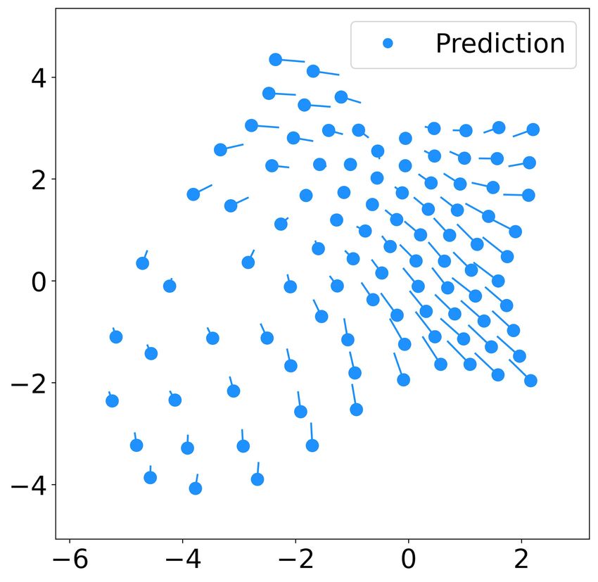
2D flocking velocity variance                         3D Boids
                                                                                     [11] Oussama KLD-POD
                                                                                                      Khatib. Real-time obstacle avoidance for manipulators and
                                                                                          mobile robots. The Int. J. of Robot. Res., 5(1):90–98, 1986.
                                                                                     [12] Akira Okubo. Dynamical aspects of animal grouping: Swarms,
                                                                                          schools, flocks, and herds. Advances in Biophysics, 22:1–94, 1986.
           Communication Range                                                       [13] Craig W Reynolds. Flocks, herds and schools: A distributed behavioral
                                                                                          model. In Proc. of the 14th annual conf. on Comput. graphics and

                                                                 Proximity Radius
                                                                                          interactive tech., pages 25–34, 1987.
                                                                                     [14] Benjamin Riviere, Wolfgang Honig, Yisong Yue, and Soon-Jo Chung.
                                                                                          Glas: Global-to-local safe autonomy synthesis for multi-robot motion
                                                                                          planning with end-to-end learning. IEEE Robot. and Automat. Lett.,
                                                                                          5(3):4249–4256, Jul 2020.
                                                                                     [15] Michael Rubenstein, Alejandro Cornejo, and Radhika Nagpal.
                                                                                          Robotics. programmable self-assembly in a thousand-robot swarm.
                                                                                          Science (New York, N.Y.), 345:795–9, 08 2014.
                                                                                     [16] SebLague. Boids. https://github.com/SebLague/Boids/
                                                                                          tree/master, 2019.
                                                                                     [17] Guanya Shi, Wolfgang Hönig, Yisong Yue, and Soon-Jo Chung.
                                 Number of Active Neighbors                         NumberNeural-swarm:     Decentralized close-proximity multirotor control using
                                                                                           of Active Neighbors
                                                                                          learned interactions. In 2020 IEEE Int. Conf. on Robot. and Automat.,
                                                                                          pages 3241–3247. IEEE, 2020.
Fig. 8. Grid search on the velocity variance using different communication           [18] Adrian Šošić, Wasiur R KhudaBukhsh, Abdelhak M Zoubir, and Heinz
radius and number of active neighbors. Small communication radius and                     Koeppl. Inverse reinforcement learning in swarm systems. arXiv
small number of active neighbors show poor velocity convergence as                        preprint arXiv:1602.05450, 2016.
expected.                                                                            [19] Herbert Tanner, Ali Jadbabaie, and George Pappas. Stable flocking
                                                                                          of mobile agents, part ii: Dynamic topology. Departmental Papers
                                                                                          (ESE), 2, 05 2003.
to reproduce flocking behavior similar to the ground truth.                          [20] Herbert G Tanner, Ali Jadbabaie, and George J Pappas. Stable flocking
                                                                                          of mobile agents, part i: Fixed topology. In 42nd IEEE Int. Conf. on
Furthermore, the learnt controllers can scale to larger swarms                            Decision and Control, volume 2, pages 2010–2015. IEEE, 2003.
to produce flocking behaviors. We has shown the effective-                           [21] Ekaterina Tolstaya, Landon Butler, Daniel Mox, James Paulos, Vijay
ness of knowledge embedding in learning decentralized con-                                Kumar, and Alejandro Ribeiro. Learning connectivity for data distri-
                                                                                          bution in robot teams. arXiv preprint arXiv:2103.05091, 2021.
trollers, and demonstrated the feasibility of learning swarm                         [22] Ekaterina Tolstaya, Fernando Gama, James Paulos, George Pappas, Vi-
behaviors from state observations alone, distinguishing our                               jay Kumar, and Alejandro Ribeiro. Learning decentralized controllers
work from prior works on imitation learning. For future                                   for robot swarms with graph neural networks. In Conf. on Robot
                                                                                          Learn., pages 671–682. PMLR, 2020.
work, we plan to implement the learnt controllers on physical                        [23] T. Vicsek. A question of scale. Nature, 411:421–421, 2001.
robot platforms to emulate swarming behaviors. In addition,                          [24] Tamás Vicsek, András Czirók, Eshel Ben-Jacob, Inon Cohen, and Ofer
we hope to employ neural networks with special properties                                 Shochet. Novel type of phase transition in a system of self-driven
                                                                                          particles. Phys. Rev. Lett., 75:1226–1229, Aug 1995.
to derive stability guarantees for the learnt controllers.                           [25] K Warburton and J Lazarus. Tendency-distance models of social
                                                                                          cohesion in animal groups. J. Theor. Biol., 150(4):473–488, June 1991.
                                      R EFERENCES                                    [26] Alexander Wikner, Jaideep Pathak, Brian Hunt, Michelle Girvan,
                                                                                          Troy Arcomano, Istvan Szunyogh, Andrew Pomerance, and Edward
 [1] C. M. Breder. Equations descriptive of fish schools and other animal                 Ott. Combining machine learning with knowledge-based modeling
     aggregations. Ecology, 35(3):361–370, 1954.                                          for scalable forecasting and subgrid-scale closure of large, complex,
 [2] Tian Qi Chen, Yulia Rubanova, Jesse Bettencourt, and David Du-                       spatiotemporal systems. Chaos, 30:053111, 05 2020.
     venaud. Neural ordinary differential equations. In Samy Bengio,
     Hanna M. Wallach, Hugo Larochelle, Kristen Grauman, Nicolò Cesa-
     Bianchi, and Roman Garnett, editors, NeurIPS, pages 6572–6583,
     2018.
 [3] G Flierl, D Grünbaum, S Levins, and D Olson. From individuals to
     aggregations: the interplay between behavior and physics. J. Theor.
     Biol., 196(4):397–454, February 1999.
 [4] Fernando Gama, Ekaterina Tolstaya, and Alejandro Ribeiro. Graph
     neural networks for decentralized controllers. In ICASSP 2021-2021
     IEEE Int. Conf. on Acoust., Speech and Signal Process., pages 5260–
     5264. IEEE, 2021.
 [5] Ramin Hasani, Mathias Lechner, Alexander Amini, Daniela Rus,
     and Radu Grosu. Liquid time-constant networks. arXiv preprint
     arXiv:2006.04439, 2020.
 [6] Philip Holmes, John L. Lumley, and Gal Berkooz. Turbulence,
     Coherent Structures, Dynamical Systems and Symmetry. Cambridge
     Monographs on Mechanics. Cambridge University Press, 1996.
 [7] Maximilian Hüttenrauch, Sosic Adrian, Gerhard Neumann, et al.
     Deep reinforcement learning for swarm systems. J. of Mach. Learn.
     Research, 20(54):1–31, 2019.
 [8] Maximilian Hüttenrauch, Adrian Šošić, and Gerhard Neumann.
     Guided deep reinforcement learning for swarm systems. arXiv preprint
     arXiv:1709.06011, 2017.
 [9] Tom Z. Jiahao, M. Ani Hsieh, and Eric Forgoston. Knowledge-
     based learning of nonlinear dynamics and chaos. arXiv preprint
     arXiv:2010.03415, 2021.
[10] George Em Karniadakis, Ioannis G. Kevrekidis, Lu Lu, Paris
     Perdikaris, Sifan Wang, and Liu Yang. Physics-informed machine
     learning. Nature Reviews Physics, 3:422–440, 06 2021.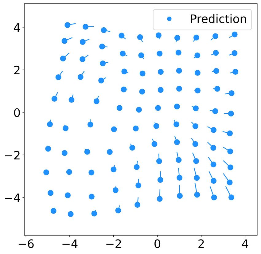
You can also read


