Dynamically-stable Motion Planning for Humanoid Robots
←
→
Page content transcription
If your browser does not render page correctly, please read the page content below
Autonomous Robots vol. 12, No. 1, pp. 105--118. (Jan. 2002)

Dynamically-stable Motion Planning for Humanoid Robots

James J. Kuffner, Jr.∗
Dept. of Mechano-Informatics, The University of Tokyo, 7-3-1 Hongo, Bunkyo-ku,
Tokyo 113-8656, JAPAN (kuffner@jsk.t.u-tokyo.ac.jp)

Satoshi Kagami
Digital Human Lab., National Institute of Advanced Industrial Science and
Technology, 2-41-6, Aomi, Koto-ku, Tokyo, 135-0064, JAPAN.
(s.kagami@aist.go.jp)

Koichi Nishiwaki, Masayuki Inaba and Hirochika Inoue
Dept. of Mechano-Informatics, The University of Tokyo, 7-3-1 Hongo, Bunkyo-ku,
Tokyo 113-8656, JAPAN ({nishi,inaba,inoue}@jsk.t.u-tokyo.ac.jp)

Abstract. We present an approach to path planning for humanoid robots that
computes dynamically-stable, collision-free trajectories from full-body posture goals.
Given a geometric model of the environment and a statically-stable desired posture,
we search the configuration space of the robot for a collision-free path that si-
multaneously satisfies dynamic balance constraints. We adapt existing randomized
path planning techniques by imposing balance constraints on incremental search
motions in order to maintain the overall dynamic stability of the final path. A
dynamics filtering function that constrains the ZMP (zero moment point) trajectory
is used as a post-processing step to transform statically-stable, collision-free paths
into dynamically-stable, collision-free trajectories for the entire body. Although we
have focused our experiments on biped robots with a humanoid shape, the method
generally applies to any robot subject to balance constraints (legged or not). The
algorithm is presented along with computed examples using both simulated and real
humanoid robots.
Keywords: Motion Planning, Humanoid Robots, Dynamics, Obstacle Avoidance

                               1. Introduction

Recently, significant progress has been made in the design and con-
trol of humanoid robots, particularly in the realization of dynamic
walking in several full-body humanoids (Hirai, 1997; Yamaguchi et al.,
1998; Nagasaka et al., 1999). As the technology and algorithms for
real-time 3D vision and tactile sensing improve, humanoid robots will
be able to perform tasks that involve complex interactions with the
environment (e.g. grasping and manipulating objects). The enabling
software for such tasks includes motion planning for obstacle avoid-
ance, and integrating planning with visual and tactile sensing data.
  ∗
    Partially supported by a Japan Society for the Promotion of Science (JSPS)
Postdoctoral Fellowship for Foreign Scholars in Science and Engineering


      c 2002 Kluwer Academic Publishers. Printed in the Netherlands.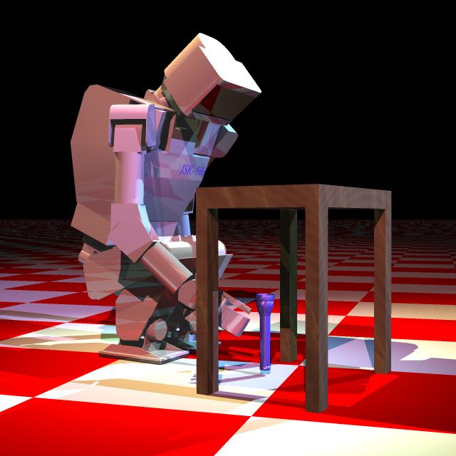
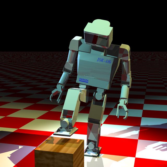
2                                 J. Kuffner e.a.

Figure 1. Dynamically-stable motion for retrieving an object (top: simulation,
bottom: real robot hardware).

Figure 2. Simulation snapshots of computed full-body trajectories.
Dynamically-stable Motion Planning for Humanoid Robots     3

To facilitate the deployment of such software, we are currently de-
veloping a graphical simulation environment for testing and debug-
ging (Kuffner et al., 2000a). Figure 2 shows images produced by our
simulation environment.
    This paper presents an algorithm for automatically generating collision-
free dynamically-stable motions from full-body posture goals. It ex-
pands upon the preliminary algorithm developed in (Kuffner et al.,
2000b), and has been tested and verified on the humanoid robot hard-
ware platform “H6”. Our approach is to adapt techniques from an ex-
isting, successful path planner (Kuffner and LaValle, 2000) by imposing
balance constraints upon incremental motions used during the search.
Provided the initial and goal configurations correspond to collision-free,
statically-stable body postures, the path returned by the planner can
be transformed into a collision-free and dynamically-stable trajectory
for the entire body. To the best of our knowledge, this represents the
first general motion planning algorithm for humanoid robots that has
also been experimentally confirmed on real humanoid robot hardware.
    Although the current implementation of the planner is limited to
body posture goals, and a fixed position for either one or both feet,
we hope to extend the method to handle more complex body pos-
ture repositioning. We believe that through the use of such kinds of
task-level planning algorithms and interactive simulation software, the
current and future capabilities of humanoid and other complex robotic
systems can be improved.
    The rest of this paper is organized as follows: Section 2 gives an
overview of previous work, Section 3 describes the planning algorithm,
Section 4 presents experimental results, and Section 5 contains a sum-
mary and outlines some areas of future work.

                            2. Background

Due to the complexity of motion planning in its general form (Reif,
1979), the use of complete algorithms (Schwartz and Sharir, 1983;
Canny, 1988) is limited to low-dimensional configuration spaces. More-
over, these algorithms are extremely difficult to implement even for sim-
ple problems(Hirukawa and Papegay, 2000; Hirukawa et al., 2001). This
has motivated the use of heuristic algorithms, many of which employ
randomization (e.g., (Barraquand and Latombe, 1990; Horsch et al.,
1994; Amato and Wu, 1996; Kavraki et al., 1996; Hsu et al., 1997; Mazer
et al., 1998; Boor et al., 1999; Kuffner and LaValle, 2000; Bohlin and
Kavraki, 2000)). Although these methods are incomplete, many have
4 J. Kuffner e.a.
been shown to find paths in high-dimensional configuration spaces with
high probability.
Motion planning for humanoid robots poses a particular challenge.
Developing practical motion planning algorithms for humanoid robots
is a daunting task given that humanoid robots typically have 30 or
more degrees of freedom. The problem is further complicated by the
fact that humanoid robots must be controlled very carefully in order
to maintain overall static and dynamic stability. These constraints
severely restrict the set of allowable configurations and prohibit the
direct application of existing motion planning techniques. Although
efficient methods have been developed for maintaining dynamic balance
for biped robots (Raibert, 1986; Vukobratovic et al., 1990; Pratt and
Pratt, 1999; Kagami et al., 2000), none consider obstacle avoidance.
2.1. Motion Planning with Dynamic Constraints
Motion planning algorithms that account for system dynamics typically
approach the problem in one of two ways:
1. Decoupled Approach: Solving the problem by first computing
a kinematic path, and subsequently transforming the path into a
dynamic trajectory.
2. State-space Formulation: Searching the system state-space di-
rectly by reasoning about the possible controls that can be applied.
The method presented in this paper adopts the first approach. Other
methods using one of these two planning strategies have been developed
for off-road vehicles(Shiller and Gwo, 1991; Cherif and Laugier, 1995),
free-flying 2D and 3D rigid bodies(LaValle and Kuffner, 1999; LaValle
and Kuffner, 2000), helicopters and satellites(Frazzoli et al., 1999), and
for a free-flying disc among moving obstacles(Kindel et al., 2000). None
of these previous methods have yet been applied to complex articulated
models such as humanoid robots. One notable exception is the VHRP
simulation software under development(Nakamura and et. al., 2000),
which contains a path planner that limits the active body degrees of
freedom for humanoid robots for simultaneous obstacle avoidance and
balance control. Since the space of possible computed motions is limited
however, this planner is not fully general.Dynamically-stable Motion Planning for Humanoid Robots 5
AutoBalancer
Motion Dynamics
Initial Planner Filter
Pose
RRT
Final Path
Pose Search
Final
Path
Solution
Collision Smoothing
Trajectory
Checker
Figure 3. Algorithm Overview.
3. Dynamically-stable Motion Planning
Our approach is to adapt a variation of the randomized planner de-
scribed in (Kuffner and LaValle, 2000) to compute full-body motions for
humanoid robots that are both dynamically-stable and collision-free.
The first phase computes a statically-stable, collision-free path, and
the second phase smooths and transforms this path into a dynamically-
stable trajectory for the entire body. An block diagram of the major
software components are shown in Figure 3.
The planning method (RRT-Connect) and its variants utilize Rapidly-
exploring Random Trees (RRTs) (LaValle, 1998; LaValle and Kuffner,
2000) to connect two search trees, one from the initial configuration and
the other from the goal. This method has been shown to be efficient
in practice and converge towards a uniform exploration of the search
space. For the second phase, the collision checker is used in conjunction
with a dynamics filter function “AutoBalancer” (Kagami et al., 2000)
in order to generate a final dynamically-stable trajectory that is also
collision-free.
3.1. Robot Model and Assumptions
We have based our experiments on an approximate model of the H6
humanoid robot (see Figure 1), including the kinematics and dynamic
properties of the links. Although we have focused our experiments on
biped robots with a humanoid shape, the algorithm generally applies to
any robot subject to balance constraints (legged or not). Aside from the
existence of the dynamic model, we make the following assumptions:
1. Environment model: We assume that the robot has access to a
3D model of the surrounding environment to be used for collision
checking. This model could have been obtained through sensors6 J. Kuffner e.a.
such as laser rangefinding or stereo vision, or given directly in
advance.
2. Initial posture: The robot is currently balanced in a collision-free,
statically-stable configuration supported by either one or both feet.
3. Goal posture: A full-body goal configuration that is both collision-
free and statically-stable is specified. The goal posture may be given
explicitly by a human operator, or computed via inverse kinematics
or other means. (e.g. for extending a limb towards a target location
or object).
4. Support base: The location of the supporting foot (or feet in
the case of dual-leg support) does not change during the planned
motion.
3.2. Problem Formulation
Our problem will be defined in a 3D world W in which the robot moves.
W is modeled as the Euclidean space 3 ( is the set of real numbers).
3.2.1. Robot
Let the robot A be a finite collection of p rigid links Li (i = 1, . . . , p)
organized in a kinematic hierarchy with Cartesian frames Fi attached
to each link. We denote the position of the center of mass ci of link
Li relative to Fi . A pose of the robot is denoted by the set P =
{T1 , T2 , . . . , Tp }, of p relative transformations for each of the links Li as
defined by the frame Fi relative to its parent link’s frame. The base or
root link transformation T1 is defined relative to some world Cartesian
frame Fworld . Let n denote the number of generalized coordinates or
degrees of freedom (DOFs) of A. A configuration is denoted by q ∈ C,
a vector of n real numbers specifying values for each of the generalized
coordinates of A. Let C be the configuration space or C-space of A. C
is a space of dimension n.
3.2.2. Obstacles
The set of obstacles in the environment W is denoted by B, where
Bk (k = 1, 2, . . .) represents an individual obstacle. We define the C-
obstacle region CB ⊂ C as the set of all configurations q ∈ C where one
or more of the links of A intersect (are in collision) with another link
of A, or any of the obstacles Bk . We also regard configurations q ∈ C
where one or more joint limits are violated as part of the C-obstacle
region CB. The open subset C \ CB is denoted by Cf ree and its closureDynamically-stable Motion Planning for Humanoid Robots 7
by cl(Cf ree ), and it represents the space of collision-free configurations
in C of the robot A.
3.2.3. Balance and Torque Constraints
Let X (q) be a vector relative to Fworld representing the global position
of the center of mass of A while in the configuration q. A configuration q
is statically-stable if: 1) the projection of X (q) along the gravity vector
g lies within the area of support SP (i.e. the convex hull of all points
of contact between A and the support surface in W), and 2) the joint
torques Γ needed to counteract the gravity-induced torques G(q) do
not exceed the maximum torque bounds Γmax . Let Cstable ⊂ C be the
subset of statically-stable configurations of A. Let Cvalid = Cstable ∩Cf ree
denote the subset of configurations that are both collision-free and
statically-stable postures of the robot A. Cvalid is called the set of
valid configurations.
3.2.4. Solution Trajectory
Let τ : I → C where I is an interval [t0 , t1 ], denote a motion trajectory
or path for A expressed as a function of time. τ (t) represents the
configuration q of A at time t, where t ∈ I. A trajectory τ is said
to be collision-free if τ (t) ∈ Cf ree for all t ∈ I. A trajectory τ is said
to be both collision-free and statically-stable if τ (t) ∈ Cvalid for all
t ∈ I. Given qinit ∈ Cvalid and qinit ∈ Cvalid , we wish to compute a
continuous motion trajectory τ such that ∀t ∈ [t0 , t1 ], τ (t) ∈ Cvalid ,
and τ (t0 ) = qinit and τ (t1 ) = qgoal . We refer to such a trajectory as a
statically-stable trajectory.
3.2.5. Dynamic Stability
Theoretically, any statically-stable trajectory can be transformed into
a dynamically-stable trajectory by arbitrarily slowing down the mo-
tion. For these experiments, we utilize the online balance compensation
scheme “AutoBalancer” described in (Kagami et al., 2000) as a method
of generating a final dynamically-stable trajectory after path smoothing
(see Section 3.5).
3.2.6. Planning Query
Note that in general, if a dynamically-stable solution trajectory exists
for a given path planning query, there will be many such solution
trajectories. Let Φ denote the set of all dynamically-stable solution
trajectories for a given problem. A planning query is as follows:
P lanner(A, B, qinit , qgoal ) −→ τ (1)
Given a model of the robot A, obstacles in the environment B, and
the initial and goal postures, the planner returns a solution trajectory8 J. Kuffner e.a.
τ ∈ Φ. If the planner fails to find a solution, τ will be empty (a null
trajectory).
Currently, we require the planning software to compute only one
solution (it returns the first one it finds). However, given a trajectory
evaluation function Γ(τ ), the planner could compute a set of candidate
trajectories Φ̄ within a given time period, and then select the best one
τbest returned so far: τbest = minΓ(τ ), τ ∈ Φ̄.
3.3. Path Search
Unfortunately, there are no currently known methods for explicitly
representing Cvalid . The obstacles are modeled completely in W, thus
an explicit representation of Cf ree is also not available. However, us-
ing a collision detection algorithm, a given q ∈ C can be tested to
determine whether q ∈ Cf ree . Testing whether q ∈ Cstable can also
be checked verifying that the projection of X (q) along g is contained
within the boundary of SP , and that the torques Γ needed to counteract
gravitational torques G(q) do not exceed Γmax .
3.3.1. Distance Metric
As with the most planning algorithms in high-dimensions, a metric ρ is
defined on C. The function ρ(q, r) returns some measure of the distance
between the pair of configurations q and r. Some axes in C are weighted
relative to each other, but the general idea is to measure the “closeness”
of pairs of configurations with a positive scalar function.
For our humanoid robot models, we employ a metric that assigns
higher relative weights to the generalized coordinates of links with
greater mass and proximity to the trunk (torso):
n
ρ(q, r) = wi ||qi − ri || (2)
i=1
This choice of metric function attempts to heuristically encode a gen-
eral relative measure of how much the variation of an individual joint
parameter affects the overall body posture. Additional experimentation
is needed in order to evaluate the efficacy of the many different metric
functions possible.
3.3.2. Planning Algorithm
We employ a randomized search strategy based on Rapidly-exploring
Random Trees (RRTs) (LaValle and Kuffner, 1999; Kuffner and LaValle,
2000). For implementation details and analysis of RRTs, the reader is
referred to the original papers or a summary in (LaValle and Kuffner,
2000). In (Kuffner et al., 2000b), we developed an RRT variant theDynamically-stable Motion Planning for Humanoid Robots 9
generates search trees using a dynamics filter function to guarantee
dynamically-stable trajectories along each incremental search motion.
The algorithm described in this article is more general and efficient
than the planner presented in (Kuffner et al., 2000b), since it does
not require the use of a dynamics filtering function during the path
search phase. In addition, it can handle either single or dual-leg support
postures, and the calculated trajectories have been verified using real
robot hardware.
The basic idea is the same as the RRT-Connect algorithm described
in (Kuffner and LaValle, 2000). The key difference is that instead of
searching C for a solution path that lies within Cf ree , the search is per-
formed in Cstable for a solution path that lies within Cvalid . In particular,
we modify the planner variant that employs symmetric calls to the
EXTEND function as follows:
1. The NEW CONFIG function in the EXTEND operation checks bal-
ance constraints in addition to checking for collisions with obstacles
(i.e. qnew ∈ Cvalid ).
2. Rather than picking a purely random configuration qrand ∈ C at
every planning iteration, we pick a random configuration that also
happens to correspond to a statically-stable posture of the robot
(i.e. qrand ∈ Cstable ).
Pseudocode for the complete algorithm is given in Figure 5. The main
planning loop involves performing a simple iteration in which each step
attempts to extend the RRT by adding a new vertex that is biased by
a randomly-generated, statically-stable configuration (see Section 3.4).
EXTEND selects the nearest vertex already in the RRT to the given
configuration, q, with respect to the distance metric ρ. Three situations
can occur: Reached, in which q is directly added to the RRT, Advanced,
in which a new vertex qnew = q is added to the RRT; Trapped, in which
no new vertex is added due to the inability of NEW CONFIG to generate
a path segment towards q that lies within Cvalid .
NEW CONFIG attempts to make an incremental motion toward q.
Specifically, it checks for the existence of a short path segment δ =
(qnear , qnew ) that lies entirely within Cvalid . If ρ(q, qnear ) < , where is
some fixed incremental distance, then q itself is used as the new configu-
ration qnew at the end of the candidate path segment δ (i.e. qnew = q).
Otherwise, qnew is generated at a distance along the straight-line
from qnear to q.1 All configurations q along the path segment δ are
1
A slight modification must be made for the case of dual-leg support. In this
case, when interpolating two stable configurations, inverse kinematics for the leg10 J. Kuffner e.a.
qtarget
q
qnew
qnear
qinit
Figure 4. The modified EXTEND operation.
checked for collision, and tested whether balance constraints are satis-
fied. Specifically, if ∀q ∈ δ(qnear , qnew ), q ∈ Cvalid , then NEW CONFIG
succeeds, and qnew is added to the tree T . In this way, the planner uses
uniform samples of Cstable in order to grow trees that lie entirely within
Cvalid .
3.3.3. Convergence and Completeness
Although not given here, arguments similar to those presented in (Kuffner
and LaValle, 2000) and (LaValle and Kuffner, 2000) can be constructed
to show uniform coverage and convergence over Cvalid .
Ideally, we would like to build a complete planning algorithm. That
is, the planner always returns a solution trajectory if one exists, and
indicates failure if no solution exists. As mentioned in Section 2, imple-
menting a practical complete planner is a daunting task for even low-
dimensional configuration spaces (see (Hirukawa and Papegay, 2000)).
Thus, we typically trade off completeness for practical performance by
adopting heuristics (e.g. randomization).
The planning algorithm implemented here is incomplete in that it
returns failure after a preset time limit is exceeded. Thus, if the planner
returns failure, we cannot conclude whether or not a solution exists for
the given planning query, only that our planner was unable to find one
in the allotted time. Uniform coverage and convergence proofs, though
only theoretical, at least help to provide some measure of confidence
that when an algorithm fails to find a solution, it is likely that no
solution exists. This is an area of ongoing research.
is used to force the relative position between the feet to remain fixed. The same s
technique is also used for generating random statically-stable dual-leg postures (see
Section 3.4).Dynamically-stable Motion Planning for Humanoid Robots 11 EXTEND(T , q) 1 qnear ← NEAREST NEIGHBOR(q, T ); 2 if NEW CONFIG(q, qnear , qnew ) then 3 T .add vertex(qnew ); 4 T .add edge(qnear , qnew ); 5 if qnew = q then Return Reached; 6 else Return Advanced; 7 Return Trapped; RRT CONNECT STABLE(qinit , qgoal ) 1 Ta .init(qinit ); Tb .init(qgoal ); 2 for k = 1 to K do 3 qrand ← RANDOM STABLE CONFIG(); 4 if not (EXTEND(Ta , qrand ) =Trapped) then 5 if (EXTEND(Tb , qnew ) =Reached) then 6 Return PATH(Ta , Tb ); 7 SWAP(Ta , Tb ); 8 Return Failure Figure 5. Pseudocode for the main loop of the algorithm. 3.4. Random Statically-stable Postures For our algorithm to work, we require a method of generating ran- dom statically-stable postures (i.e. random point samples of Cstable ). Although it is trivial to generate random configurations in C, it is not so easy to generate them in Cstable , since it encompasses a much smaller subset of the configuration space. In our current implementation, a set Qstable ⊂ Cstable of N samples of Cstable is generated as a preprocessing step. This computation is specific to a particular robot and support-leg configuration, and need only be performed once. Different collections of stable postures are saved to files and can be loaded into memory when the planner is initialized. Although stable configurations could be generated “on-the-fly” at the same time the planner performs the search, pre-calculating Qstable is preferred for efficiency. In addition, multiple stable-configuration set files for a particular support-leg configuration can be saved indepen- dently. If the planner fails to find a path after all N samples have been
12                                 J. Kuffner e.a.

removed from the currently active Qstable set, a new one can be loaded
with different samples. 2 .

3.4.1. Single-leg Support Configurations
For configurations that involve balancing on only one leg, the set Qstable
can be populated as follows:
 1. The configuration space of the robot C is sampled by generating a
    random body configuration qrand ∈ C.3
 2. Assuming the right leg is the supporting foot, qrand is tested for
    membership in Cvalid (i.e. static stability, no self-collision, and joint
    torques below limits).
 3. Using the same sample qrand , a similar test is performed assuming
    the left leg is the supporting foot.
 4. Since most humanoid robots have left-right symmetry, if qrand ∈
    Cvalid in either or both cases, we can “mirror” qrand to generate
    stable postures for the opposite foot.

3.4.2. Dual-leg Support Configurations
It is slightly more complicated to generate statically-stable body con-
figurations supported by both feet at a given fixed relative position.
In this case, populating Qstable is very similar to the problem of sam-
pling the configuration space of a constrained closed-chain system (e.g.
closed-chain manipulator robots or molecular conformations (LaValle
et al., 1999; Han and Amato, 2000)). The set Qstable is populated with
fixed-position dual-leg support postures as follows:
 1. As in the single-leg case, the configuration space of the robot C is
    sampled by generating a random body configuration qrand ∈ C.
 2. Holding the right leg fixed at its random configuration, inverse
    kinematics is used to attempt to position the left foot at the re-
    quired relative position to generate the body configuration qright .
    If it succeeds, then qright is tested for membership in Cvalid .
  2
     Since our humanoid robot H6 has 33 DOF, storing a 4-byte float for each
joint variable corresponds to roughly 1.2MB of storage per N = 10, 000 sample
configurations. However, this memory usage can be significantly reduced by adopting
fixed-point representations for the joint variables. This has not implemented in our
current planner.
   3
     This can be done by simply independently sampling all joint variables. Alterna-
tively, one can assemble body configurations from collections of canonical postures
for each limb. Our implementation uses the latter approach, since sampling all joints
independently tends to generate rather strange or unnatural postures.
Dynamically-stable Motion Planning for Humanoid Robots 13
Figure 6. Dual-leg and single-leg stable postures for H5 (perspective view).
3. An identical procedure is performed to generate qlef t by holding
the left leg fixed at its random configuration derived from qrand ,
using inverse kinematics to position the right leg, and testing for
membership in Cvalid .
4. If either qright ∈ Cvalid or qlef t ∈ Cvalid , and the robot has left-right
symmetry, additional stable postures can be derived by mirroring
the generated stable configurations.
A sample series of dual-leg and single-leg stable postures for the H5
humanoid robot are shown in Figure 6 (perspective view), Figure 7
(front view), and Figure 8 (left view). Sample dual-leg and single-leg
stable postures for the H6 humanoid robot are shown in Figure 9.
3.5. Trajectory Generation
If successful, the path search phase returns a continuous sequence of
collision-free, statically-stable body configurations. All that remains
is to calculate a final solution trajectory τ that is dynamically-stable
and collision-free. Theoretically, any given statically-stable trajectory
can be transformed into a dynamically-stable trajectory by arbitrarily
slowing down the motion. However, we can almost invariably obtain a
smoother and shorter trajectory by performing the following two steps:14 J. Kuffner e.a.
.
.
.
Figure 7. Dual-leg and single-leg stable postures for H5 (front view).
Figure 8. Dual-leg and single-leg stable postures for H5 (left view).Dynamically-stable Motion Planning for Humanoid Robots 15
Figure 9. Dual-leg and single-leg stable postures for H6 (perspective view).
3.5.1. Smoothing
We smooth the raw path by making several passes along its length,
attempting to replace portions of the path between selected pairs of
configurations by straight-line segments in Cvalid .4 This step typically
eliminates any potentially unnatural postures along the random path
(e.g. unnecessarily large arm motions). The resulting smoothed path
is transformed into an input trajectory using a minimum-jerk model
(Flash and Hogan, 1985).
3.5.2. Filtering
A dynamics filtering function is used in order to output a final, dynamically-
stable trajectory. We use the online balance compensation scheme de-
scribed in (Kagami et al., 2000), which enforces constraints upon the
center of gravity projection and zero moment point (ZMP) trajectory
in order to maintain overall dynamic stability. The overall body posture
is adjusted iteratively in order to compensate for any violation of the
constraints.
The constrained output trajectory is calculated by posing the bal-
ance compensation problem as an optimization problem under rea-
sonable assumptions about the input motion trajectory (for details,
see (Kagami et al., 2000)). The output configuration of the filter is
guaranteed to lie in Cstable . Collision-checking is used to verify that the
final output trajectory lies in Cvalid . The filter is invoked repeatedly: if
a collision is detected, the speed of the input trajectory is made slower.
4
When interpolating dual-leg configurations, inverse kinematics is used to keep
the relative position of the feet fixed.16 J. Kuffner e.a.
Figure 10. Dynamically-stable planned trajectory for a crouching motion.
If no collision is detected, the speed is increased, filtered, and checked
again for collision.
Although this method has generated satisfactory results in our ex-
periments, it is by no means the only option. Other ways of generating
dynamically-stable trajectories from a given input motion are also po-
tentially possible to apply here (e.g. (Yamaguchi et al., 1998; Nakamura
and Yamane, 2000)). It is also possible to employ variational techniques,
or apply algorithms for computing time-optimal trajectories (Shiller
and Dubowsky, 1991). Calculating the globally-optimal trajectory ac-
cording to some cost functional based on the obstacles and the dynamic
model is an open problem, and an area of ongoing research.
4. Experiments
This section presents some preliminary experiments performed on a 270
MHz SGI O2 (R12000) workstation. We have implemented a prototype
planner in C++ that runs within a graphical simulation environment
(Kuffner et al., 2000a). An operator can position individual joints or
use inverse kinematics to specify body postures for the virtual robot.
The filter function can be run interactively to ensure that the goal
configuration is statically-stable. After specifying the goal, the plan-
ner is invoked to attempt to compute a dynamically-stable trajectory
connecting the goal configuration to the robot’s initial configuration
(assumed to be a collision-free, stable posture).
Figure 10 shows a computed dynamically-stable motion for the H5
robot moving from a neutral standing position to a low crouching
posture.
We have tested the output trajectories calculated by the planner
on an actual humanoid robot hardware platform. The “H6” humanoid
robot (33-DOF) is 137cm tall and weighs 51kg (including 4kg of bat-
teries).
Several full-body motion trajectories were planned. Figure 1 shows
a computed dynamically-stable motion for the H6 robot moving fromDynamically-stable Motion Planning for Humanoid Robots 17
.
Figure 11. Dynamically-stable crouching trajectory for retrieving an object from
beneath an obstacle
a neutral standing position to a low crouching position in order to
retrieve an object from beneath a chair. Figure 11 shows a different
view of the real robot executing the same motion. This motion was
executed “open-loop” on the robot, but was accurate enough to allow
the robot to successfully pick up the object from the floor. In the future,
we hope to use the stereo vision system mounted in the robot’s head
in order to visually servo such object manipulation motions.
Two single-leg examples were calculated. Figure 12 shows a motion
for positioning the right leg above the top of an obstacle while balancing
on the left leg. The motion in Figure 13 was not executed on the real
robot, but is interesting in that it involves reaching for an object placed
on top of a cabinet while avoiding both the cabinet and the shelves
behind the robot. The robot is required to balance on one leg in order
to extend the arm far enough to reach the obstacle on the table.
Each of the scenes contains over 9,000 triangle primitives. The 3D
collision checking software used for these experiments was the RAPID
library based on OBB-Trees developed by the University of North Car-
olina(Gottschalk et al., 1996). The total wall time elapsed in solving
these queries ranges from under 30 seconds to approximately 11 min-
utes. A summary of the computation times for repeated runs of 25 trials
each is shown in Table I.18 J. Kuffner e.a.
Figure 12. Positioning the right foot above an obstacle while balancing on the left
leg. (top: simulation, bottom: actual hardware).
Figure 13. Reaching for an object atop a cabinet while avoiding obstacles and
balancing on the right leg.
Table I. Performance statistics (N = 25 trials).
Task Description Computation Time (seconds)
min max avg stdev
H5 - Crouch near table 176 620 304 133
H6 - Reach under chair 171 598 324 138
H6 - Lift leg over box 26 103 48 21
H6 - Reach over table 194 652 371 146Dynamically-stable Motion Planning for Humanoid Robots 19
5. Discussion
This paper presents an algorithm for computing dynamically-stable
collision-free trajectories given full-body posture goals. Although we
have focused our experiments on biped robots with a humanoid shape,
the algorithm is general and can be applied to any robot subject to
balance constraints (legged or not). There are many potential uses
for such software, with the primary one being a high-level control
interface for automatically computing motions to solve complex tasks
for humanoid robots that involve simultaneous obstacle-avoidance and
balance constraints.
The limitations of the algorithm form the basis for our future work:
− the current implementation of the planner can only handle a fixed
position for either one or both feet. The ability to chage the base
of support, or perform “dynamic” transitions such as jumping or
hopping from one foot to the other would be an exciting improve-
ment.
− The effectiveness of different configuration space distance metrics
needs to be investigated.
− We currently have no method for integrating visual or tactile feed-
back.
Acknowledgements
We thank Fumio Kanehiro and Yukiharu Tamiya for their efforts in
developing the AutoBalancer software library. We are grateful to Hiro-
hisa Hirukawa and Steven LaValle for helpful discussions. This research
is supported in part by a Japan Society for the Promotion of Science
(JSPS) Postdoctoral Fellowship for Foreign Scholars in Science and
Engineering, and by JSPS Grant-in-Aid for Research for the Future
(JSPS-RFTF96P00801).
References
Amato, N. and Y. Wu: 1996, ‘A Randomized Roadmap Method for Path and Ma-
nipuation Planning’. In: Proc. IEEE Int. Conf. Robot. & Autom. (ICRA). pp.
113–120.
Barraquand, J. and J.-C. Latombe: 1990, ‘Robot Motion Planning: A distributed
representation approach’. Int. J. Robot. Res. 10(6), 628–649.20 J. Kuffner e.a. Bohlin, R. and L. Kavraki: 2000, ‘Path Planning Using Lazy PRM’. In: Proc. IEEE Int. Conf. Robot. & Autom. (ICRA). Boor, V., M. Overmars, and A. van der Stappen: 1999, ‘The Gaussian Sampling Strategy for Probabilistic Roadmap Planners’. In: Proc. IEEE Int. Conf. Robot. & Autom. (ICRA). Canny, J.: 1988, The Complexity of Robot Motion Planning. Cambridge, MA: MIT Press. Cherif, M. and C. Laugier: 1995, ‘Motion Planning of Autonomous Off-Road Vehicles Under Physical Interaction Constraints’. In: Proc. IEEE Int. Conf. Robot. & Autom. (ICRA). Flash, T. and N. Hogan: 1985, ‘The coordination of arm movements: an experimen- tally confirmed mathematical model’. J. Neurosci. 5(7), 1688–1703. Frazzoli, E., M. Dahleh, and E. Feron: 1999, ‘Robust Hybrid Control for Autonomous Vehicles Motion Planning’. Technical report, Laboratory for Information and Decision Systems, Massachusetts Institute of Technology, Cambridge, MA. Technical report LIDS-P-2468. Gottschalk, S., M. C. Lin, and D. Manocha: 1996, ‘OBBTREE: A Hierarchical Structure for Rapid Interference Detection’. In: SIGGRAPH ’96 Proc. Han, L. and N. M. Amato: 2000, ‘A Kinematics-Based Probabilistic Roadmap Method for Closed Chain Systems’. In: Proc. Int. Workshop Alg. Found. Robot.(WAFR). Hirai, K.: 1997, ‘Current and future perspective of Honda humanoid robot’. In: Proc. IEEE/RSJ Int. Conf. Intell. Robot. & Sys. (IROS). pp. 500–508. Hirukawa, H., B. Mourrain, and Y. Papegay: 2001, ‘A Symbolic-Numeric Silhouette Algorithm’. In: Proc. IEEE/RSJ Int. Conf. Intell. Robot. & Sys. (IROS). Hirukawa, H. and Y. Papegay: 2000, ‘Motion Planning of Objects in Contact by the Silhouette Algorithm’. In: Proc. IEEE Int. Conf. Robot. & Autom. (ICRA). pp. 722–729. Horsch, T., F. Schwarz, and H. Tolle: 1994, ‘Motion Planning for Many Degrees of Freedom : Random Reflections at C-Space Obstacles’. In: Proc. IEEE Int. Conf. Robot. & Autom. (ICRA). pp. 3318–3323. Hsu, D., J.-C. Latombe, and R. Motwani: 1997, ‘Path Planning in Expansive Configuration Spaces’. Int. J. Comput. Geom. & Appl. 9(4-5), 495–512. Kagami, S., F. Kanehiro, Y. Tamiya, M. Inaba, and H. Inoue: 2000, ‘AutoBalancer: An Online Dynamic Balance Compensation Scheme for Humanoid Robots’. In: Proc. Int. Workshop Alg. Found. Robot.(WAFR). Kavraki, L., P. Švestka, J. C. Latombe, and M. H. Overmars: 1996, ‘Probabilistic Roadmaps for Path Planning in High-Dimensional Configuration Space’. IEEE Trans. Robot. & Autom. 12(4), 566–580. Kindel, R., D. Hsu, J. Latombe, and S. Rock: 2000, ‘Kinodynamic Motion Planning Amidst Moving Obstacles’. In: Proc. IEEE Int. Conf. Robot. & Autom. (ICRA). Kuffner, J., S. Kagami, M. Inaba, and H. Inoue: 2000a, ‘Graphical Simulation and High-Level Control of Humanoid Robots’. In: Proc. IEEE/RSJ Int. Conf. Intell. Robot. & Sys. (IROS). Kuffner, J. and S. LaValle: 2000, ‘RRT-Connect: An Efficient Approach to Single- Query Path Planning’. In: Proc. IEEE Int. Conf. Robot. & Autom. (ICRA). Kuffner, J., S.Kagami, M. Inaba, and H. Inoue: 2000b, ‘Dynamically- stable Mo- tion Planning for Humanoid Robots’. In: IEEE-RAS Int. Conf. Human. Robot. (Humanoids). Boston, MA. LaValle, S. and J. Kuffner: 1999, ‘Randomized Kinodynamic Planning’. In: Proc. IEEE Int. Conf. Robot. & Autom. (ICRA).
Dynamically-stable Motion Planning for Humanoid Robots              21

LaValle, S. and J. Kuffner: 2000, ‘Rapidly-Exploring Random Trees: Progress and
   Prospects’. In: Proc. Int. Workshop Alg. Found. Robot.(WAFR).
LaValle, S., J. Yakey, and L. Kavraki: 1999, ‘A Probabilistic Roadmap Approach
   for Systems with Closed Kinematic Chains’. In: Proc. IEEE Int. Conf. Robot. &
   Autom. (ICRA).
LaValle, S. M.: 1998, ‘Rapidly-Exploring Random Trees: A New Tool for Path
   Planning’. TR 98-11, Computer Science Dept., Iowa State Univ.
Mazer, E., J. M. Ahuactzin, and P. Bessière: 1998, ‘The Ariadne’s Clew Algorithm’.
   J. Artificial Intell. Res. 9, 295–316.
Nagasaka, K., M. Inaba, and H. Inoue: 1999, ‘Walking pattern generation for a
   humanoid robot based on optimal gradient method’. In: Proc. IEEE Int. Conf.
   Sys. Man. & Cyber.
Nakamura, Y. and et. al.: 2000, ‘V-HRP: Virtual Humanoid Robot Platform’. In:
   IEEE-RAS Int. Conf. Human. Robot. (Humanoids).
Nakamura, Y. and K. Yamane: 2000, ‘Interactive Motion Generation of Humanoid
   Robots via Dynamics Filter’. In: Proc. of First IEEE-RAS Int. Conf. on
   Humanoid Robots.
Pratt, J. and G. Pratt: 1999, ‘Exploiting Natural Dynamics in the Control of a 3D
   Bipedal Walking Simulation’. In: In Proc. of Int. Conf. on Climbing and Walking
   Robots (CLAWAR99).
Raibert, M.: 1986, Legged Robots that Balance. Cambridge, MA: MIT Press.
Reif, J. H.: 1979, ‘Complexity of the mover’s problem and generalizations’. In: Proc.
   20th IEEE Symp. on Foundations of Computer Science (FOCS). pp. 421–427.
Schwartz, J. T. and M. Sharir: 1983, ‘On the ‘Piano Movers’ Problem: II. General
   Techniques for computing topological properties of real algebraic manifolds’.
   Advances in applied Mathematics 4, 298–351.
Shiller, Z. and S. Dubowsky: 1991, ‘On Computing Time-Optimal Motions of
   Robotic Manipulators in the Presence of Obstacles’. IEEE Trans. Robot. &
   Autom. 7(7).
Shiller, Z. and R. Gwo: 1991, ‘Dynamic Motion Planning of Autonomous Vehicles’.
   IEEE Trans. Robot. & Autom. 7(2), 241–249.
Vukobratovic, M., B. Borovac, D. Surla, and D. Stokie: 1990, Biped Locomotion:
   Dynamics, Stability, Control, and Applications. Berlin: Springer-Verlag.
Yamaguchi, J., S. Inoue, D. Nishino, and A. Takanishi: 1998, ‘Development of a
   bipedal humanoid robot having antagonistic driven joints and three dof trunk’.
   In: Proc. IEEE/RSJ Int. Conf. Intell. Robot. & Sys. (IROS). pp. 96–101.
You can also read