Lecture 4: RL from Deep Learning Perspectives - EPFL Summer School on Data Science, Optimization and Operations Research August 15-20, 2021

EPFL Summer School on Data Science, Optimization and Operations Research
 August 15-20, 2021

 Lecture 4: RL from Deep Learning Perspectives

 Niao He, D-INFK, ETH Zurich

Recap: Reinforcement Learning Approaches

 • Value-based RL
 Actor ◦ Estimate the optimal value function ∗ ( , )
 Value-based Critic Policy-based ◦ Example: Q-learning

 • Policy-based RL
 ◦ Search directly the optimal policy ∗ (⋅ | )
 ◦ Example: Policy Gradient Method

 Model-based
 • Model-based RL
 ◦ First estimate the model , and then do planning

 2

Outline of Lecture Series

 Focus:
 Provably convergent “deep” RL methods

 Lecture 1 Introduction to RL

 RL from Control Perspectives
 Lecture 2
 - Value-based RL
 o RL with nonlinear function approximation

 Lecture 3 RL from Optimization Perspectives o RL with neural network approximation
 - Policy-based RL

 RL from Deep Learning Perspectives
 Lecture 4
 - Deep RL

 Lecture 5 RL from Game Perspectives

 3

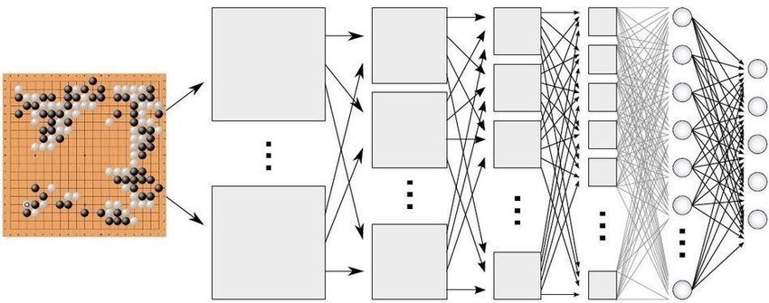
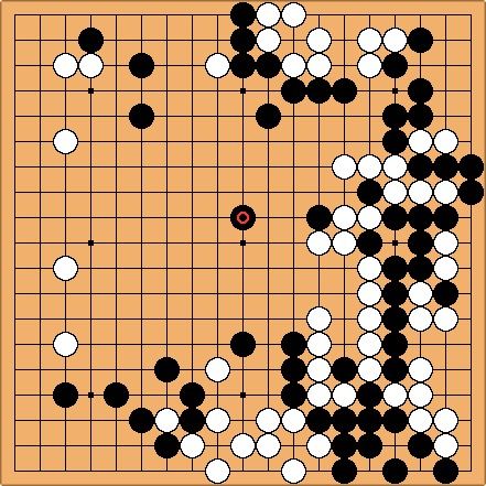
The Grand Challenge
 Chess: 10$%& Go: 3"#$

• Large state space, policy space

 State 
 Action " 
 Learn parameter
 " , ∈ !
 ( ≪ | |)
 " | 
 " , # , 

 Using neural network approximation seems a must.
 AI = RL + DL?
 4

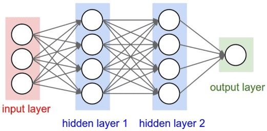
Neural Networks

• Nested composition of (learnable) linear transformation with (fixed) nonlinear activation functions
 !m
 A single-hidden-layer neural network f (x; w, α) = αi σ(wiT x)
 i=1

 $,$
 $
 Activation function ⋅ :
 $
 • Identity: = 
 %
 • Sigmoid: =
 $
 $'()*(,-)
 0 • Tanh: = tanh 
 • Rectified linear unit: = max(0, )
 1
 1,0

 Input layer hidden layer output
 ( nodes)
 5

Deep Neural Networks

• More hidden layers, different activation functions, more general graph structure ….

 Feed forward network Convolutional network

 Residual network Recurrent network

 … 

 6

Representation Power - why neural networks?

 Shallow networks are universal Benefits of depth
 approximators

 • Any continuous function on bounded domain • A deep network cannot be approximated by a
 can be approximated arbitrarily well by a one- reasonably-sized shallow network.
 hidden layer network with nonconstant and
 increasing continuous activation function.
 • There exists ReLU networks with ( ) nodes in 2
 [Cybenko, 1989; Hornik et al.,1989; Barron, 1993] hidden layers which cannot be approximated by 1-
 hidden-layer networks with less than 2! nodes.
 [Eldan and Shamir, 2015]
 • Number of neurons can be large.
 • There exists a function with " layers and width 2
 which requires width 2# to approximate with
 ( ) layers. [Telgarsky 2015,2016]

 7

Training with Neural Networks

 • Gradient vanishing or exploding
 ReLU activation, gradient clipping
 • Overfitting
 regularization techniques
 (dropout, early stopping, etc.) • Nonconvexity
 noisy gradient

 • Ill-conditioning
 adaptive gradient methods
 (Adam, AdaGrad, RMSprop, etc.)

Deep Reinforcement Learning

• Using (deep) neural networks to represent
 ◦ Value function
 ◦ Policy
 ◦ Model
 Actor
 Value-based Critic Policy-based

 Model-based

 9

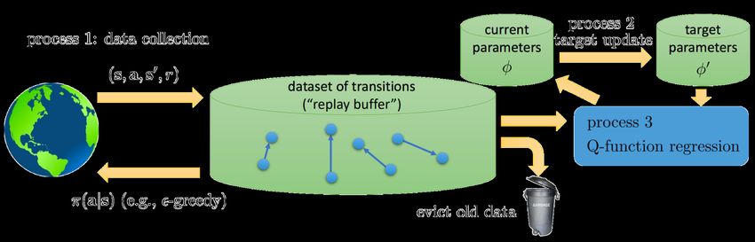
Deep Value-based and Actor-critic RL

 • Deep Q-Learning

 Q∗ (s, a) ≈ Q(s, a; w)
 ! "
 " " − 2
 min L(w) := E(s,a,s! ,r)∼D (r + γ max
 !
 Q(s , a ; w ) − Q(s, a; w))
 w a

 • Stabilizing training: (prioritized) experience replay, target network, double learning, dueling network.

Figure source: EE-618 at EPFL 10

The Deadly Triad?

 Network capacity
 Target networks
 Overestimation

 Of

 Of
 g

 f-p

 g
 pi n
 Multi-step returns

 f-p
 pi n
 oli

 oli
 p

 p
 ra

 cy

 ra

 cy
 Prioritization
 st

 st
 D
 ot

 D
 at

 ot

 at
 Bo

 a

 Bo

 a
 Function Approximation Function Approximation

 Q-learning with function DQN successfully learnt to play
 Theory Practice
 approximation could diverge. many Atari 2600 games.
 [Barto & Sutton, 2018] [van Hasselt et al, 2018]

 11

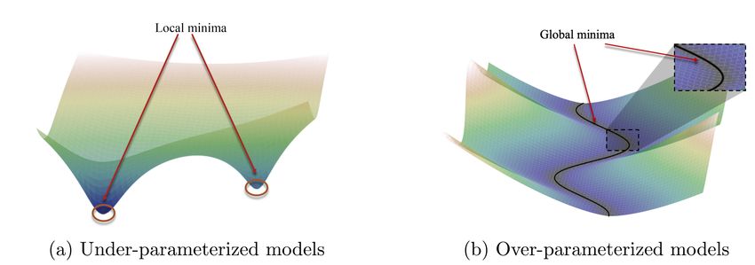
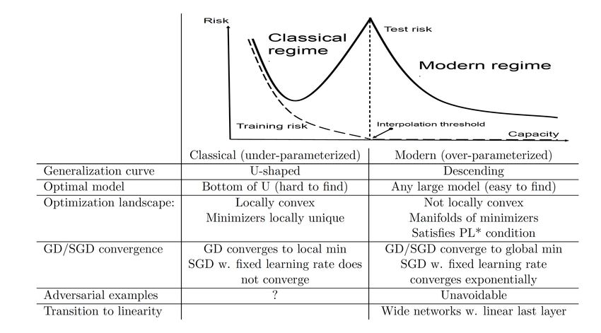
Wisdom from modern deep learning theory

Mikhail Belkin. Fit without fear: remarkable mathematical phenomena of deep learning through the prism of Interpolation, 2021. 12

The optimization landscape

 Extensive work:
 Jacot et al. 2018; Li and Liang 2018; Du et al. 2018; Allen-Zhu et al. 2018; Oymak and Soltanolkotabi
 2019; Zou et al. 2018; Chizat and Bach 2019; Ji and Telgarsky 2019a; Z. Chen et al. 2019; Arora et al.
 2019; Cao and Gu 2020; ……

Liu et al. Loss landscapes and optimization in over-parameterized non-linear systems and neural networks, 2021. 13

The neural tangent kernel (NTK)

• Supervised learning: find a model parameter that fits the training data
 f (xi ; w∗ ) ≈ yi , i = 1, . . . , n

 1!
 n
 minm L(w) := (f (xi ; w) − yi )2
 w∈R 2 i=1

• Neural tangent kernel:
 Kij (w) = !∇w f (xi ; w), ∇w f (xj ; w)#
 Kij (w0 ) = Ew0 ∼N (0,Im ) !∇w f (xi ; w0 ), ∇w f (xj ; w0 )#

• Kernel matrix: " ≽ 0 if is sufficiently large

 14

Key insight behind the scene

• Gradient flow:
 dw(t)
 = −∇L(w(t))
 dt & ≽ &, for random & and large
 u(t) = f (w(t); x) − y = ( )

 du(t) 1
 = −K(w(t))u(t) 123 − 123 & = ,
 dt 
 for ∈ 

• PL* condition
 ( ) ≻ 

 !∇L(w)!2 = (f (w; x) − y)T K(w)(f (w; x) − y)
 ≥ 2 · λmin (K(w)) · L(w) / converges to global optima

 15

Supervised Learning vs. RL

• Common features: learning from experience and generalize
 ◦ SL: given $ , $ $%&,…,) , learn best in hypothesis class
 ◦ RL: given $ , $ , $ $%&,…,) , learn best ( , ) or ∗ = arg min ( , ).
 +

• Distinguishing features of RL:
 ◦ Lack of supervisor, only a reward signal
 ◦ Delayed feedback
 ◦ Non-i.i.d. data
 ◦ Difficulty with data reuse

 16

Notation Recap
 MDP ( , , , , , )

 State value function:

 State-action value function:

 Optimal value function:

 Optimal policy:

 Bellman equation: V π (s) = Ea∼π(s) R(s, a) + γEs! ∼P (·|s,a) V π (s" )
 ! "

 Bellman optimality:

 Policy gradient:

 State visitation distribution:

 17

TD Learning with Neural Network Approximation

• Value function approximation: = ∈ = hidden layer

 input layer
 1 , . output
 > ; , = E $ $- 
 $%& >
 ( ; , )

• Symmetric Initialization:

 $ = − $.,/" ∼ −1,1 , $ 0 = $.,/" 0 ∼ (0, ! )

• Neural TD Learning:

 + 1 = ( ) + / / + >/ /.& − >/ / ∇0 >/ ( / )

 18

Optimization Perspective

 Minimizing mean-square Bellman error (MSBE):
 )
 min $∼& 8 ; , − + $4 |$ 8 ( ; , 
 #

• TD Learning can be viewed as a stochastic semi-gradient method.
• With neural network approximation, the MSBE objective becomes non-convex.
• Approximation error between 8 ; , and true value function ( ).

 Goal: Can we achieve >- − ≤ ?
 • Sample complexity (required number of samples)?
 • Network complexity (required number of neurons)?

 19

Existing Theory

• TD Learning with linear function approximation
 ◦ Finite-time analysis of TD with projection: [Bhandari et al., 2019]
 ◦ Finite-time analysis of TD without projection: [Srikant & Ying, 2019]
 ◦ Finite-time analysis under i.i.d. setting: [Dalal et al., 2018], [Lakshminarayanan & Szepesvári, 2018]

• (Stochastic) Gradient Descent with two-layer overparametrized neural network
 ◦ Infinite-width limit ( → ∞): [Jacot et al., 2018], [Chizat et al., 2019]
 ◦ GD with polynomial width: [Du et al., 2018] , [Oymak and Soltanolkotabi, 2019], [Arora et al., 2019]
 ◦ SGD with polylogarithmic width (classification only): [Ji & Telgarsky, 2020]

 Key Challenges:
 • Massive overparameterization (poly in | |) is not suitable for TD Learning
 • Drift of the network parameter || − 0 ||

 20

Neural Tangent Kernel
 * /
• Recall 8 ; , = ∑+ ,. 
 + ,-* ,

 1 ,
 > ; , ≈ > ; 0 , + E $ $- 0 ≥ 0 - [ $ − $ (0)]
 $%&

 1 ,
 > ; , ≈ E $ $- 0 ≥ 0 - $
 $%&

• Neural Tangent Kernel:
 , = 05∼1(", 46) [ ". ≥ 0 ". ≥ 0 . ]
 ◦ The NTK is a universal kernel.
 ◦ The corresponding RKHS is dense in the continuous function space defined on a compact set.

• Assumption: = . " ⋅ ". ≥ 0 , where sup ( ) ) ≤ ̅ < ∞.
 0

 21

Neural TD Learning with Regularization

 Algorithm 1: Projection-Free NTD Algorithm 2: Max-Norm NTD

 + 1 = + ⋅ / $ + 1 = Proj2 0! 3 ,4 [ $ + ⋅ /$ ]

 Regularization: Early stopping Regularization: Max-norm
 = ( ,̅ , ) || $ − $ 0 ||" ≤ / 
 (Ji & Telgarsky, ’19, Li et al., ‘20) for SL (Srivastava, ‘14, Goodfellow, ’13) for SL

 $ + 1/2

 $ + 1
 $ 
 / 
 $ 0

 22

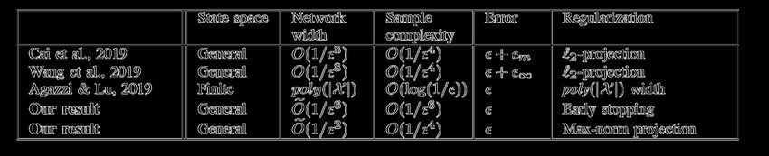
Convergence of Neural TD

 Assumption: ( ⋅ ) ∈ 1.6 (dense in cont. functions over a compact state space (Ji et al., ’19))

 8. − & 1ℰ ≤ where ℰ > 1 − 

 Algorithm 1: Projection-Free NTD Algorithm 2: Max-Norm NTD
 Sample complexity: = ̅ / # Sample complexity: = / 7

 Network width: = ̅ / # Network width: = ( )/ %

 Projection radius: > ̅

 Here ̅ is the bound of the NTK norm of ⋅ .

 23

Highlight

• Some regularization + modest overparameterization à convergence to true value function

More expressive power Faster convergence

 Projection-free NTD [Cai et al., ’19] Max-norm NTD
 (Early stopping) (ℓ" -reg.) (ℓ5 -reg)

 24

Lyapunov Drift Analysis

• Minimum norm solution:
 Z = [ , 0 + , 8
 
 #8 "
 ],∈[+]
 +
 Note that ∇ 8 ; 0 , . Z → , → ∞.
 
• Lyapunov function: Z
 = − )
 )

 <
• Stopping time: = inf > 0: , − , 0 ) > for some .
 +

• Drift bound:

 ) ?9 A@ :
 > @
 = + 1 − ≤ −2 1 − 8= − &
 +O ) + , for < 
 +

 25

Drift Bound

• Recall + 1 = + = ,

 ! = ! ⋅ ∇" &! ! ; ( ) ,
 g
 +1 − "
 "
 g
 = − "
 " + 2 /- g + " /
 − "
 " ! = ! + &! !#$ − &! ! .

• Bound the second term
 g ]
 [ /- − 

 = [ / ⋅ ∇0 >/ / ; ( ) - g ]
 − 
 - - -
 = / ⋅ >/ / ; − / + / − ∇ >/ / ; 0 g + ∇ >/ / ; 0
 g − ∇ >/ / ; 
 g
 
 " ̅ 
 ≤ − 1 − >/ − ≤ ≤ 
 6 

 26

Extensions and Open Questions

• Extensions of Neural TD Learning
 ◦ Markovian setting
 ◦ Extended feature vector
 ◦ Smooth activation functions

• Open Questions
 ◦ Beyond two-layers, can we achieve reduced overparameterization bound?
 ◦ Beyond two-layers, under what conditions can we achieve global convergence?
 ◦ Is early stopping or regularization necessary?
 ◦ Extension to deep Q-learning to find optimal policy?
 ◦ How to integrate RL with general nonlinear function approximation in a more principled manner?

 27

Optimization-based RL Algorithms

• Bellman-residual-minimization methods
 ◦ Residual gradient algorithm [Baird, 1995] Rich theory and gradient-based
 algorithms for nonconvex optimization
 ◦ Gradient TD [Sutton et al., 2009]
 ◦ Least-Squares Policy Iteration [Antos et al., 2006]
 ◦ SBEED [Dai et al., 2018] Exploitation of off-policy data

• Linear programming-based methods Adaptation to neural network
 approximation
 ◦ Stochastic primal-dual method [Chen & Wang, 2016] [Lee & He, 2018]
 ◦ Dual actor-critic [Dai et al., 2017]
 Extensibility (safety, multi-agent RL, etc)
 ◦ Primal-dual stochastic mirror descent [Jin & Sidford, 2020]
 ◦ Logistic Q-learning [Bas-Serrano et al., 2021]

• Policy gradient methods
 ◦ Natural policy gradient method (NPG) [Kakade, 2001]
 ◦ Trust region policy optimization (TRPO) [Schulman et al., 2015]
 ◦ Proximal policy optimization algorithm (PPO) [Schulman et al., 2017]
 ◦ Entropy-regularized policy gradient methods and actor-critic algorithms

 28

Revisit Bellman Optimality Equation

 • Recall the Bellman optimality equation:

 • Equivalently:

 ◦ The -operator is highly nonsmooth and causes instability when function approximation is used.

 29

Smoothing the -Operator

• Introduce entropic regularization to Bellman optimality equation,

 ◦ , = − ∑ log is the entropy, > 0 is the smoothness parameter

• The smoothed Bellman operator is also a -contraction.

Bellman Residual Minimization

• Minimizing mean-squared smoothed Bellman error:
 Swimmer Hopper

 (CSO):

 (Min-Max SO):

 Convergent off-policy RL algorithm
 with nonlinear function approximation
 [Dai et al., ICML 2018]

 Caveat: require solving nonconvex-(non)concave min-max optimization!
 31

Linear-programming-based Method

• LP formulation:

 (Primal policy):
 (Dual policy):

 (Min-Max SO):

 Convergent off-policy RL algorithm
 w/o function approximation
 [Dai et al., 2017; Donghwan and H., 2019]

 Caveat: lack of duality; require solving nonconvex-(non)concave min-max optimization!
 32

Summary
• Understanding the convergence and generalization of deep RL from modern deep learning theory
• Principled approaches for RL with neural network approximation

 Value-based methods Optimization-based methods Policy-based methods
 • Neural TD learning • Bellman Residual Minimization • Neural Policy Gradient
 • Neural Q-learning • Linear Programming • Neural Actor Critic

 Open Questions
 • Benefits of depth and different architectures?
 • Nonconvex min-max optimization?
 • Regularization and sample complexity?

 33

Reference

• [Cayci, Satpathi, H., Srikant, 2021] Sample Complexity and Overparameterization Bounds for Temporal
 Difference Learning with Neural Network Approximation. arXiv preprint arXiv:2103.01391, 2021.

• [Dai et al., 2018] SBEED: Convergent Reinforcement Learning with Nonlinear Function Approximation. ICML
 2018.

• [Du et al., 2019] Gradient Descent Provably Optimizes Over-parameterized Neural Networks. ICLR 2019.

• [Fan et al., 2020] A Theoretical Analysis of Deep Q-Learning. arXiv: 1901.00137, 2019.

 34