Locality Relationship Constrained Multi-view Clustering Framework
←
→
Page content transcription
If your browser does not render page correctly, please read the page content below
IEEE TRANSACTIONS ON MULTIMEDIA, VOL. XXX, NO. XX, 2021                                                                                    1

                                                  Locality Relationship Constrained Multi-view
                                                             Clustering Framework
                                                                                      Xiangzhu Meng, Wei Wei∗ , and Wenzhe Liu

                                            Abstract—In most practical applications, it’s common to utilize          producing satisfied performance by integrating the diversity
                                         multiple features from different views to represent one object.             information among different views. An easy yet effective
                                         Among these works, multi-view subspace-based clustering has                 way is to concatenate all views as one common view, then
                                         gained extensive attention from many researchers, which aims
                                         to provide clustering solutions to multi-view data. However,                utilize traditional single view methods to solve the clustering
arXiv:2107.05073v1 [cs.CV] 11 Jul 2021

                                         most existing methods fail to take full use of the locality                 task. However, this manner not only neglects the specific
                                         geometric structure and similarity relationship among samples               statistical property in each view , but cannot take full use of
                                         under the multi-view scenario. To solve these issues, we propose            the consistency and complementary information from multiple
                                         a novel multi-view learning method with locality relationship               views.
                                         constraint to explore the problem of multi-view clustering, called
                                         Locality Relationship Constrained Multi-view Clustering Frame-                  To solve above issues, plenty of multi-view clustering meth-
                                         work (LRC-MCF). LRC-MCF aims to explore the diversity,                      ods have been widely proposed in the past ten years. A class
                                         geometric, consensus and complementary information among                    of representative multi-view methods [16–20] investigate to
                                         different views, by capturing the locality relationship information         construct one common latent view shared by all views, which
                                         and the common similarity relationships among multiple views.               can integrate the diversity and complementary information
                                         Moreover, LRC-MCF takes sufficient consideration to weights
                                         of different views in finding the common-view locality structure            from different views into the common view and then partition
                                         and straightforwardly produce the final clusters. To effectually            it into the ideal groups. For example, Auto-Weighted Multiple
                                         reduce the redundancy of the learned representations, the low-              Graph Learning (AMGL)[17] method automatically assigns an
                                         rank constraint on the common similarity matrix is considered               ideal weight for each view in integrating multi-view informa-
                                         additionally. To solve the minimization problem of LRC-MCF, an              tion according to the importance of each view. Nevertheless,
                                         Alternating Direction Minimization (ADM) method is provided
                                         to iteratively calculate all variables LRC-MCF. Extensive exper-            they cannot guarantee the complementarity information among
                                         imental results on seven benchmark multi-view datasets validate             different views so that rich multi-view information cannot
                                         the effectiveness of the LRC-MCF method.                                    be further fully utilized. Therefore, another class of multi-
                                           Index Terms—Multi-view clustering, Locality Relationship                  view clustering methods are proposed to further discover
                                         Constraint, Alternating Direction Minimization                              the complementary information among different views. These
                                                                                                                     works based on Canonical Correlation Analysis (CCA) [21]
                                                                                                                     and Hilbert-Schmidt Independence Criterion (HSIC) [22] are
                                                                  I. I NTRODUCTION                                   two classes of representative multi-view clustering methods.
                                            With the rapid development of the information era, one                   The former [23–25] employs CCA to project the pairwise
                                         common object can usually be represented by different view-                 views into the common subspace by maximizing the corre-
                                         points [1, 2]. For example, the document (or paper) can be                  lation between two views, and the latter [26–28] explores
                                         represented by different languages [3, 4]. Generally, multiple              complementary information based on HSIC term by mapping
                                         views can contain more meaningful and comprehensive in-                     variables into a reproducing kernel Hilbert space. Apart from
                                         formation than single view, which provide some knowledge                    these above works, co-training strategy [29, 30] is also con-
                                         information not involved in single view. The fact can show                  sidered as an effective tool to enforce different views to learn
                                         that, properly using multi-view information is beneficial for               from each other. Unfortunately, these methods may produce
                                         improving the practical performance in most situations. How-                unsatisfactory results when the gap of different views is
                                         ever, most traditional methods mainly focus on the single                   varying large. Although such methods have achieved excellent
                                         view, which cannot be directly used to deal with multi-view                 performances in some situations, most of them always focus
                                         data. Therefore, multi-view learning [5–7] methods has been                 on either the intrinsic structure information in each view or
                                         proposed in different tasks, such as classifications [8–10],                geometric structures from other views. To discover the geo-
                                         clustering [11, 12], etc. Notably, multi-view clustering [13–               metric structures information in multi-view data, those works
                                         15] has become an important research field, which aims at                   [31–35] have been developed to learn the intrinsic structure
                                                                                                                     in each view. However, the geometric structures information
                                         X. Meng is with Center for Research on Intelligent Perception and Comput-   in these works usually depend on artificial definition, which
                                         ing, Institute of Automation, Chinese Academy of Sciences, Beijing, China
                                         (xiangzhu.meng@cripac.ia.ac.cn).                                            cannot learn the geometric relation among samples from multi-
                                         W. Wei is with Center for Energy, Environment & Economy Research,           view data. To sum up, multi-view clustering is still an open
                                         Tourism Management School of Zhengzhou University, Zhengzhou, China         yet challenging problem.
                                         (weiwei123@zzu.edu.cn).
                                         W. Liu is with the School of Computer Science and Technology, Dalian            To solve these issues, we propose a novel multi-view
                                         University of Technology, Dalian, China (liuwenzhe@mail.dlut.edu.cn).       learning method, called Locality Relationship Constrained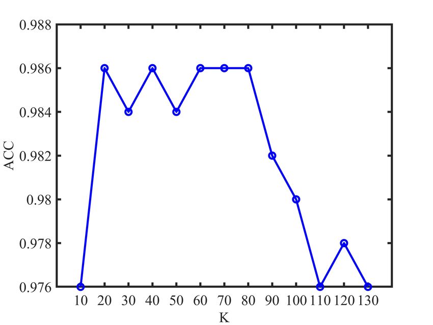
IEEE TRANSACTIONS ON MULTIMEDIA, VOL. XXX, NO. XX, 2021                                                                                     2

Multi-view Clustering Framework (LRC-MCF), to explore the                                 II. R ELATED WORKS
problem of multi-view clustering. LRC-MCF simultaneously              In this section, we review two classical multi-view learning
explores the diversity, geometric, consensus and complemen-         methods, including Auto-Weighted Multiple Graph Learning,
tary information among different views, which attempts to           and Co-regularized Multi-view Spectral Embedding.
capture the locality relationship information in each view,
and then fuse the locality structure information in all views
                                                                    A. Auto-Weighted Multiple Graph Learning
into one common similarity relationships among multiple
views. In this way, we not only take use of the diversity             Auto-Weighted Multiple Graph Learning (AMGL)[17] is a
and geometric information among multiple views, but enforce         multi-view framework based on the standard spectral learn-
difference different views to learn with each other by the          ing, which can be used for multi-view clustering
                                                                                                                n         and semi-    o
common similarity relationships. Note that there is differ-         supervised classification tasks. Let X v = xv1 , xv2 , . . . , xvN
ent clustering performance for each view, thus LRC-MCF              denote the features set in the vth view. AMGL aims to find
adaptively assign the suitable weights for different views          the common embedding U ∈ RN ×k as follows:
in finding the common-view locality structure and straight-                                  M q
forwardly produce the final clusters. To effectually reduce
                                                                                             X
                                                                                        max        tr(U T Lv U )                     (1)
the redundancy of the learned representations, the low-rank                               U ∈C
                                                                                                 v=1
constraint on the common similarity matrix is additionally                   v
                                                                    where L denotes the normalized graph Laplacian matrix in
considered. To solve the minimization problem of LRC-MCF,
                                                                    the vth view, trace(·) denotes the trace of the matrix, and k is
the optimization algorithm based on the alternating direction
                                                                    the number of clusters. C deontes the different constraints in
minimization strategy is provided to iteratively calculate all
                                                                    the Eq. (1), if C is U T U = I, the framework is used to solve
variables LRC-MCF. Finally, extensive experimental results on
                                                                    the clustering tasks; if C contains the labels information, the
seven benchmark multi-view datasets show the effectiveness
                                                                    framework is also used for the semi-supervised classification
and superiority of the LRC-MCF method.
                                                                    task. Applying the Lagrange Multiplier method to solve the
                                                                    Eq. (1), the adaptive weight mechanism is derived to allocate
                                                                    suitable weights for different views. Therefore, the multi-view
A. Contributions                                                    framework can be transformed as the following problem:
  The major contributions of this paper can be summarized                                        M
                                                                                                 X                T
as follows:                                                                               max          αv tr(U Lv U )                     (2)
                                                                                          U ∈C
                                                                                                 v=1
  •   LRC-MCF simultaneously explores the diversity, geomet-
      ric, consensus and complementary information among            where
                                                                                                q
      different views, by capturing the locality relationship in-
                                                                                        αv = 1/ 2 tr(U T Lv U )                           (3)
      formation and the common similarity relationships among
      multiple views.
                                                                    According to the Eq. (1), if the vth view is good, then
  •   LRC-MCF takes sufficient consideration to weights of                T
                                                                    tr(U Lv U ) should be small, and thus the learned weight
      different views in finding the common-view locality             v
                                                                    α for the vth view is large. Correspondingly, a bad view will
      structure, and adds the low-rank constraint on the com-
                                                                    be also assigned a small weight. Therefore, AMGL optimizes
      mon similarity matrix to effectually reduce the redun-
                                                                    the weights meaningfully and can obtain better result than the
      dancy of the learned representations.
                                                                    classical combination approach which assigns equal weight to
  •   To solve the minimization problem of LRC-MCF, an
                                                                    all the views.
      Alternating Direction Minimization (ADM) method is
      provided to iteratively calculate all variables LRC-MCF,
      which can convergence in limited iterations.                  B. Co-regularized Multi-view Spectral Clustering
  •   The experimental results on seven benchmark datasets             Co-regularized Multi-view Spectral Clustering (Co-reg)[36]
      demonstrate effectiveness and superiority of LRC-MCF,         is a spectral clustering algorithm under multiple views, which
      which outperforms its counterparts and achieves compa-        achieves this goal by co-regularizing the clustering hypotheses
      rable performance.                                            across views. Co-reg aims to propose a spectral clustering
                                                                    framework for multi-view setting. To achieve this goal, Co-reg
                                                                    works with the cross-view assumption that the true underlying
B. Organization                                                     clustering should assign corresponding points in each view
                                                                    to the same cluster. For the example of two-view case for
   The rest of the paper is organized as follows: in Section II,    the ease of exposition, the cost function for the measure of
we provide briefly some related methods which have attracted        disagreement between two clusters of the learned embedding
extensive attention; in Section III, we describe the construc-      U v and U w in the pth view and the qth view could be defined
tion procedure of LRC-MCF and optimization algorithm for            as follows:
LRC-MCF; in Section IV, extensive experiments on text and                                                                             2
image datasets demonstrate the effectiveness of our proposed                        v     w            KU v                KU w
                                                                              D (U , U ) =                    2       −           2       (4)
approach; in Section V, the conclusion is put forth finally.                                       kKU v kF               kKU w kF    F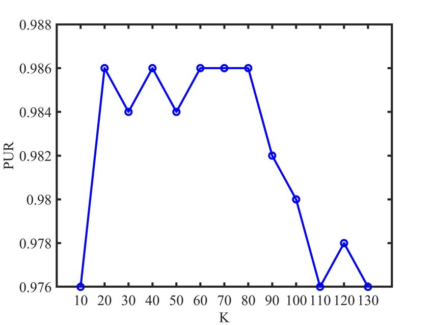
IEEE TRANSACTIONS ON MULTIMEDIA, VOL. XXX, NO. XX, 2021 3
where KU v and KU w denote the similarity matrix for the Inspired by sparse representation method, we attempt to
pth view and the qth view, respectively. For the convenience additionally add the sparsity constraint on S v , which encour-
of solving the solution, linear kernel is chosen as the similarity ages the similarity matrix S v to have more zero elements.
measure. Co-reg builds on the standard spectral clustering by Usually, L0 or L1 norm could be used to implement the
appealing to the co-regularized framework, which makes the sparsity constraint, but this manner might neglect the local
clustering relationships on different views agree with each structure in representation space. Based on the fact that the
other. Therefore, combining Eq. (4) with the spectral clustering sample point could be inflected by its some nearest neighbors,
objectives of all views, we could get the following joint we use the local structure information to construct the sparsity
maximization problem for M views: constraint for S v , thus we can obtain the following equation
based on locality relationship:
M
X T X
min tr(U v Lv U v ) + λ D (U v , V w ) N X
X N
2
U 1 ,U 2 ,...,U M
v=1 1≤v6=w≤M min
v
d(xvi , xvj )Si,j
v
+ λ kS v kF
S
T i=1 j=1
s.t. U v U v = I,1 ≤ v ≤ M (8)
(5) s.t.si,j ≥ 0, 1T Siv
v
=1
v
Si,j = 0, if xvj / N (xvi )
∈
where the first term is the spectral clustering objectives, λ
is a the non-negative hyperparameter to trade-off the spectral where N (xvi ) denotes the K nearest neighbors set of xvi .
clustering objectives and the spectral embedding disagreement
terms across different views. In this way, Co-reg implements B. Multi-view information integration
a spectral clustering framework for multi-view setting.
For the multi-view setting, a naive way is to incorporate all
views directly according to the definition in Eq. (8), which
III. T HE P ROPOSED A PPROACH can be expressed as follows:
N X
M X N M
A. Locality relationship preserving X X 2
min
v
d(xvi , xvj )Si,j
v
+λ kS v kF
Given two samples andxvi xvi
in the vth view, the distance S
v=1 i=1 j=1 v=1
(9)
between two samples is denoted as d(xvi , xvj ), which is usually v
s.t.∀v, Si,j ≥ 0, 1T Siv = 1
calculated by Mahalanobis distance. Eulidean distance, L1 - v
norm, etc. Intuitively, the distance between samples reflects the Si,j = 0, if xvj ∈
/ N (xvi )
relationship between samples, which is of vital importance to However, this manner is equal to solve the problem for
construct the local geometric structure for the set of samples. all views separately, which will fail to integrate multi-view
For the vth view, conventional similarity relationship between features and make favorable use of the complementary infor-
v d(xv ,xv )
two samples is usually defined as Si,j = exp (− iσ j ), mation from multiple views. To solve this issue, we firstly
where σ is a hyper-parameter. However, one major disad- make such hypothesis that similarities among the instances in
vantage of this manner is that the hyper-parameter is hard each view and the centroid view should be consistent under the
to set in practice due to the noise and outliers in the data. novel representations. This hypothesis means that all similarity
Therefore, how to learn the suitable similarity matrix is of vital matrices from multiple views should be consistent with the
importance. Meanwhile, the learnt similarity matrix should be similarity of the centroid view, which is implemented by
subject to such a condition that a smaller distance between aligning the similarities matrix computed from the centroid
two data points corresponds to a large similarity value, and a view and the vth view. Therefore, we utilize the following
larger distance between two data points corresponds to a small cost function as a measurement of disagreement between the
similarity value. Toward this end, we model the problem as centroid view and the vth view:
follows: 2
D (S ∗ , S v ) = kS ∗ − S v kF (10)
N X
X N
2
min
v
d(xvi , xvj )Si,j
v
+ λ kS v kF where S ∗ denotes the similarity matrix in the centroid view.
S
i=1 j=1
(6)
To integrate rich information among different features, we
v
s.t.Si,j ≥0 could obtain the following optimization problem by adding up
cost function in the Eq. (10) from all views:
where the second term is a regularization term on S v , and
M
λ is a hyperparameter to balance these two terms. To further X 2
analyze S v , we add the normalization on S v in the Eq. (6), min
∗
kS ∗ − S v kF
S
v=1
i.e. 1T svi = 1, which makes the second term constant. Then, ∗
(11)
the above problem can be transformed as follows: s.t. Si,j ≥ 0, 1T Si∗ = 1
N X
X N
2
min
v
d(xvi , xvj )Si,j
v
+ λ kS v kF In most practical applications, different views cannot play
S
i,j=1 j=1 (7) the same role in fusing different similarity matrixes. To reflect
v
s.t.Si,j ≥ 0, 1T Siv =1 the importance of different features in integrating multi-view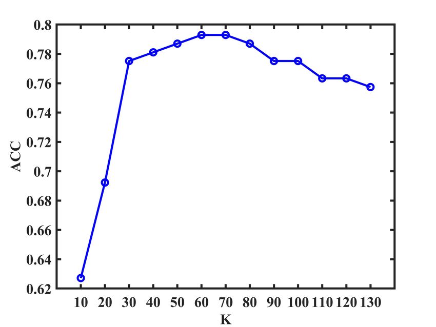
IEEE TRANSACTIONS ON MULTIMEDIA, VOL. XXX, NO. XX, 2021 4
information, we can obtain the following optimization problem D. Optimization process
by allocating ideal weights w for all views: Obviously, all the variables in the Eq. (14) are coupled
M together, thus solving the multi-view clustering problem to
X 2
min wv kS ∗ − S v kF optimize all variable at once is still challenging. In addition,
w,S ∗ the constraints are not smooth. To overcome these issues, we
v=1
(12)
s.t. ∗
Si,j ≥ 0, 1T Si∗ = 1 propose a novel algorithm based on the Alternating Direc-
tion Minimization strategy. Under the assumption that other
w ≥ 0, 1T w = 1
v
variables have been obtained, we can calculate S ∗ via the
where wv can reflect the importance of the vth view in Augmented Lagrange Multiplier scheme. That is to say, one
obtaining the common similarity matrix S ∗ . variable is updated when the other variables are fixed, which
inspires us to develop an alternating iterative algorithm to solve
problem. The specific updated rules are shown below:
C. Multi-view clustering based on Locality relationship pre- Fixing w and S ∗ , update S v : When w and S ∗ are given,
serving graph matrix S v in the Eq. (14) is independent. Thus, we can
update S v one by one, formulated as follows:
To simultaneously exploit the diversity and consensus infor-
N X
N
mation among different views, we can obtain the multi-view X 2
min d(xvi , xvj )Si,j
v
+ λ kS v kF
clustering framework by combining the Eq. (8) and Eq. (12): v
S
i=1 j=1
2 (15)
+ wv kS ∗ − S v kF
M X
N X
N M v
X X 2 s.t. Si,j ≥ 0, 1T Siv = 1
min d(xvi , xvj )Si,j
v
+λ kS v kF
v
w,S ∗ ,{S v }
v=1 i=1 j=1 v=1 Si,j = 0, if xvj ∈
/ N (xvi )
M
X r 2 It’s easy to find that the above equation is independent
+ (wv ) kS ∗ − S v kF
for different i. Thus, we can solve the following problem
v=1 (13) separately for each Siv :
∗
s.t. Si,j > 0, 1T Si∗ = 1
N
wv > 0, 1T w = 1 X 2
min d(xvi , xvj )Si,j
v
+ λ kS v kF
∀v, svi,j > 0, 1T svi = 1 vS
j=1
v
Si,j = 0, if xvj ∈
/ N (xvi ) + wv kSi∗ − Siv k2
2 (16)
v
s.t. Si,j ≥ 0, 1T Siv = 1
Our paper aims to solve the final clustering problem, i.e.,
v
producing the clustering result directly on the unified graph Si,j = 0, if xvj ∈
/ N (xvi )
matrix S ∗ without an additional clustering algorithm or step.
By relaxing the constraint, we can transform the above equa-
So far, the unified graph matrix S ∗ cannot tackle this problem.
tion as follows: Siv :
Now we give an efficient and yet simple solution to achieve
this goal by imposing a rank constraint on the graph Laplacian N
X 2
matrix L∗ of the unified matrix S ∗ . The works imply that if min
v
d(xvi , xvj )Si,j
v
+ λ kSiv k2
S
rank(L∗ ) = N − c, the corresponding S ∗ is an ideal case j=1
(17)
2
based on which the data points are partitioned into c clusters + wv kSi∗ − Siv k2
directly. Thus, there is no need to run an additional clustering v
s.t. Si,j ≥ 0, 1T Siv = 1
algorithm on the unified graph matrix S ∗ to produce the final
clusters. Motivated by this theorem, we add a rank constraint Using Lagrangian multiplier method and KKT condition to
v
to the above problem. Then our final multi-view clustering solve it, we can obtain the following solution for Si,j :
model can be formulated as follows:
v
−d(xvi , xvj ) + 2wv + 2λη
M X
N X
N M Si,j = (18)
X X 2 2λ + 2wv
min
∗
d(xvi , xvj )Si,j
v
+λ kS v kF
w,S ,{S v }
v=1 i=1 j=1 v=1 where η is Lagrangian coefficient of the constraint 1T svi = 1.
M
X Considering the locality constraint that svi,j must be equal to 0
2
+ wv kS ∗ − S v kF if xvj ∈/ N (xvi ), we can further solve the η and λ in the above
v=1 equation. Finally, we can get the following updated rule to
∗
s.t. Si,j > 0, 1T Si∗ = 1 (14) solve S v :
∗ ∗
wv > 0, 1T w = 1 d(xv v v v v
i ,xî )−d(xi ,xj )+2w )(Si,j −Si,î )
K(d(xv ,xv )−2S ∗ )+PK (2wv )S ∗ −d(xv ,xv )) ,
v
∀v, Si,j > 0, 1T Siv = 1 v
Si,j =
i î i,î k=1 i,j i j
if xvj ∈ N (xvi )
v
= 0, if xvj ∈
/ N (xvi )
Si,j
0, otherwise
rank(L∗ ) = N − c (19)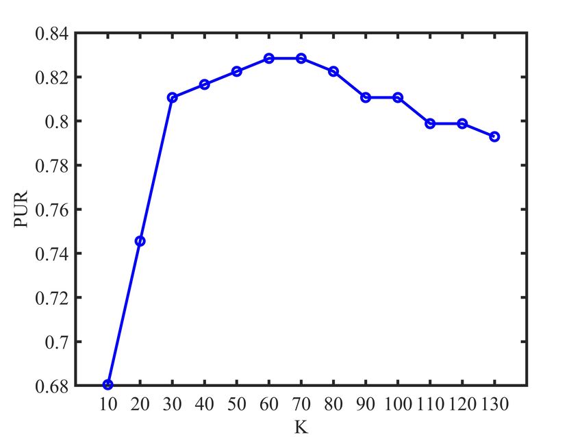
IEEE TRANSACTIONS ON MULTIMEDIA, VOL. XXX, NO. XX, 2021 5
where î is the index of the (K + 1)th nearest neighbor of xi . Fixing {S v } and S ∗ , update w: When {S v } and S ∗ are
In this way, we can sequentially update the similarity matrix given, the objective function on w can be reduced as follows:
in each view by the above equation. M
Fixing w and {S v }, update S ∗ : When w and {S v } are
X 2
min wv kS ∗ − S v kF
given, the objective function in the Eq. (14) on S ∗ can be w
v=1
(26)
reduced as follows: s.t. w > 0, 1T w = 1
v
M
X r 2 The solution to w in the above equation is wv = 1 corre-
min
∗
(wv ) kS ∗ − S v kF sponding to the min(D (S ∗ , S v )) over different views, and
S
v=1
(20)
∗
wv = 0 otherwise. This solution means that only one view is
s.t. Si,j > 0, 1 T
Si∗ ∗
= 1, rank(L ) = N − c finally selected by this method. Therefore, the performance of
this method is equivalent to the one from the best view. This
It is difficult to solve the above equation because the constraint
solution does not meet our objective on exploring the comple-
rank(L∗ ) = N − c is nonlinear. Inspired by the work that
mentary property of multiple views to get a better embedding
L∗ is positive
Pc semi-definite, the low-rank constraint can be than based on a single view. To avoid this phenomenon, we
achieved i=1 θi = 0, where θi is the ith smallest eigenvalue r
adopt a simple yet effective trick, i.e. we set wv ← (wv )
of L∗ . According to Ky Fan’s theorem [37], we can obtain the
with r ≥ 1. In this way, the novel objective function can be
following equation by combining it with the above equation:
transformed as follows:
M
X M
r 2
(wv ) kS ∗ − S v kF + βtr(F L∗ F T )
X r 2
min
∗
min (wv ) kS ∗ − S v kF
S ,F
v=1
(21) w (27)
v=1
∗
s.t. Si,j > 0, 1 T
Si∗ = 1, F F T
=I s.t. wv ≥ 0, 1T w = 1
To solve the above equation, we iteratively solve S ∗ and F . By using the Lagrange multiplier γ to take the constraint
When F is fixed, the above equation on S ∗ can be transformed 1T w = 1 into consideration, we get the following Lagrange
as follows: function:
M M
M X r 2
X
min
X
v r
(w ) kS ∗ −
2
S v kF + βtr(F L∗ F T ) L(w, γ) = (wv ) kS ∗ − S v kF − γ( wv − 1) (28)
∗
S
v=1
(22) v=1 v=1
∗
s.t. Si,j > 0, 1T Si∗ = 1 By setting the partial derivatives of L(w, γ) with respect to
w and γ to zeros, w can be calculated as follows:
For solving S ∗ , the above equation can be rewritten as follows:
2 1/(1−r)
(kS ∗ − S v kF )
M X
N N wv = P 1/(1−r)
(29)
X
v r ∗ v 2
X
∗ 2 M ∗ v 2
min
∗
(w ) (Si,j − Si,j ) +β Si,j (fi∗ − fj∗ ) i=1 (kS − S kF )
si
v=1 i,j=1 i,j=1 2
∗
Obviously, kS ∗ − S v kF is a non-negative scala, thus we have
s.t. Si,j > 0, 1T Si∗ =1 wv ≥ 0 naturally. According to the above equation, we have
(23) the following understanding for r in controlling w. When
r → ∞, different wv will be close to each other. When
Let e denote the Eulidian distance matrix of F , i.e. ei,j =
2 r → ∞, only wv = 1 corresponding to the minimum
(fi∗ − fj∗ ) , it’s easy to prove that the above optimal problem
value of D (S ∗ , S v ) over different views, and wv = 0
is equal to the following equation:
otherwise. Therefore, the selection of r should be based on
M X
N 2 the complementary property of all views.
X β
min Si∗ − Siv + r ei To sum up, we can iteratively solve the all variables in Eq.
∗si
v=1 i=1
(wv ) 2 (24) (14) according to the aforementioned descriptions, which ob-
∗
s.t. Si,j > 0, 1T Si∗ =1 tain a local optimal solution of LRC-MCF. For the convenient
of readers, we summarize the whole optimization process in
The Eq. (24) is a standard quadratic constraint problem, which the Algorithm 1. Since problem is not a joint convex problem
can be effectively solved by optimization tools. When S ∗ is of all variables, obtaining a globally optimal solution is still
fixed, the above equation on F can be simplified as follows: an open problem. We solve problem using an alternating
algorithm (as Algorithm 1). As each sub-problem is convex
min tr(F L∗ F T ) and we find the optimal solution of each sub-problem, thus
F (25)
s.t.F F T = I the algorithm converges because the objective function reduces
with the increasing of the iteration numbers. In particular,
Obviously, L∗ is a symmetric positive-definite matrix. Based with fixed other variables, one optimal variable can reduce the
on the Ky-Fan theory, F in Eq.(25) has a global optimal value of the objective function. Moreover, we will empirically
solution, which is given as the eigenvectors associated with validate the convergence of our algorithm in the following
the c smallest eigenvalues of L∗ . experiments.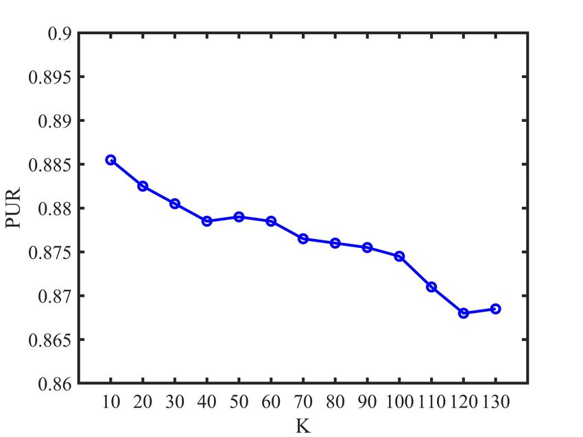
IEEE TRANSACTIONS ON MULTIMEDIA, VOL. XXX, NO. XX, 2021                                                                                           6

  Algorithm 1: The optimization procedure for LRC-                     A. Datasets
  MCF                                                                     To comprehensively demonstrate the effectiveness of the
   Input: Multi-view features {X v , ∀1 ≤ v ≤ M }, the                 proposed LRC-MCF, we perform all multi-view cluster-
            hyper-parameters α and β, the distance metric              ing methods on seven benchmark multi-view datasets, in-
            function d(·, ·), the number of clustering c.              cluding BBC1 , BBCSport2 , 3Source3 , Cora4 , Handwritten5 ,
 1 for v=1:M do                                                        HW2sources6 , and NGs7 . BBC is a documents dataset con-
 2     Initialize d(xvi , xvj ) according to the distance              sisting of 685 documents, where each document is received
        metric function d(·, ·).                                       from BBC news corpora, corresponding to the sports news
 3     Initialize S v by solving the Eq. (8).                          in five topical areas, and when we treat each topical area
 4     Initialize wv = 1/M.                                            as one view, BBC can be regarded as a dataset with five
 5 end                                                                 views; BBCSport consists of 544 documents received from
              v        v               ∗
 6 Fixing w and S , initialize S by solving the Eq.                    the BBC Sport website, where each document is corresponding
    (24).                                                              to the sports news in five topical areas, and BBCSport is
 7 while all variables not converged do                                also can be regarded as a dataset with five views; 3Source
 8     for v=1:M do                                                    contains 169 news, collected from three well-known news
 9          Fixing wv and S ∗ , update S v by the Eq. (19).            organizations (including BBC, Reuters, and Guardian), where
10          Fixing S v and S ∗ , update wv by the Eq. (29).            each news is manually annotated with one of six labels;
11     end                                                             Cora contains 2708 scientific publications of seven categories,
12     Fixing wv and S v , update S ∗ by solving the Eq.               where each publication document can be described by content
        (24).                                                          and citation, thus Cora could be considered as a two-view
13     Fixing S ∗ , update F by solving the Eq. (25).                  benchmark dataset; Handwritten is a hand-written dataset
14 end                                                                 consisting of 2000 samples, where each sample is represented
   Output: The common similarity relationship matrix                   by six different features; HW2sources is a benchmark dataset
              S∗.                                                      from the UCI repository, including 2000 samples, which is
                                                                       collected two sources including Mnist hand-written digits and
                                                                       USPS hand-written digits; NGs is a dataset consisting of
E. Computational Complexity Analysis                                   500 documents, where each document is pre-proposed by
                                                                       three different methods and manually annotated with one
   To clearly show the efficiency of LRC-MCF, we provide its           of five labels. For convenience, we summarize the statistic
computational complexity analysis in this section. Obviously,          information on these datasets in Table I.
the computational complexity to solve the all variables in
Eq. (14) is mainly dependent on the following five parts:              TABLE I: The summary information of benchmark datasets
the computational complexity to initialize all variables in              Datasets                Samples             Classes            Views
Eq. (14) is O(M N 2 d + M N K), where d is the computa-
                                                                         BBC                        685                 5                 4
tional complexity to the distance metric function d(·, ·); the
                                                                         BBCSport                   544                 5                 2
computational complexity to update S v by the Eq. (19) is
O(M N K); the computational complexity to update S ∗ by                  3Source                    169                 6                 3
solving the Eq. (24) is O(CN ); the computational complexity             Cora                      2708                 7                 2
to update F is O(CN 2 ); the computational complexity to                 Handwritten               2000                 10                6
update wv by the Eq. (29) is O(M N 2 ). Accordingly, the                 HW2sources                2000                 10                2
overall computational complexity of Algorithm 1 is about                 NGs                        500                 5                 3
O(M N 2 d + M N K + T (M N K + CN 2 + CN + M N 2 )),
where T is the iteration times of the alternating optimization
procedure in the Algorithm 1.
                                                                       B. Compared Methods
                                                                         We compare the proposed LRC-MCF with the following
                     IV. E XPERIMENTS                                  baseline methods on the above seven benchmark datasets,
                                                                       including two single-view learning methods, one feature con-
  To evaluate the effectiveness and superiority of the proposed        catenation method, and eight multi-view learning methods.
LRC-MCF, we conduct comprehensive clustering experiments               The detail information of these comparing methods can be
on seven benchmark multi-view datasets in this section. Firstly,       summarized as follows:
we introduce the details of the experiments, including bench-      1   http://mlg.ucd.ie/datasets/segment.html
mark datasets, compared methods, experiment setting, and           2   http://mlg.ucd.ie/datasets/segment.html
                                                                   3
evaluation metrics. Then, we perform all methods on different          http://mlg.ucd.ie/datasets/3sources.html
                                                                   4   3http://lig-membres.imag.fr/grimal/data.html
multi-view datasets to evaluate the performance of LRC-MCF         5   https://archive.ics.uci.edu/ml/datasets/One-hundred+palnt+pecies+leaves+data
and analysis the experimental results. Finally, we empirically         +set
demonstrate the sensitivity analysis and the parameter analysis    6   https://cs.nyu.edu/roweis/data.html
of LRC-MCF.                                                        7   http://lig-membres.imag.fr/grimal/data.html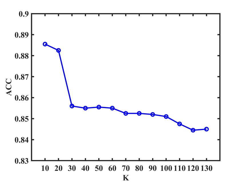
IEEE TRANSACTIONS ON MULTIMEDIA, VOL. XXX, NO. XX, 2021                                                                               7

  •   Single-view learning methods: Spectral Clustering (SC)          methods for given datasets to obtain the corresponding repre-
      [38] first computes the affinity between each pair of           sentations and then utilize K-means clustering [45] to cluster
      points to construct the similarity matrix, and then make        all samples; for the proposed LRC-MCF, we directly perform
      use of the spectrum (eigenvalues) of the similarity matrix      the clustering process on the common similarity relationship
      to perform dimensionality reduction before clustering           matrix S ∗ solved by the Algorithm 1. Since the clustering [45]
      in fewer dimensions; Graph regularized Non-negative             algorithm is known to be sensitive to initialization, We run all
      Matrix Factorizatio (GNMF) [39] aims to yield a natural         methods repeatedly 10 times and then obtain the mean value
      parts-based representation for the data and jointly dis-        of all indicators for all methods. It’s worthy noting that all
      cover the intrinsic geometrical and discriminating struc-       experiments are performed in the same environment.
      ture of the data space.                                            Given the label information of all samples, three validation
  •   Feature concatenation method: We first concatenates             metrics are adapted to validate the performance of clustering
      the features of all views and then employs the traditional      method, including accuracy (ACC), normalized mutual infor-
      clustering method to obtain the clustering results.             mation (NMI), and purity (PUR). Specifically, ACC is defined
  •   Multi-view learning methods: Canonical Correlation              as follows:
      Analysis (CCA) [21] is utilized to deal with multi-view                                   PN
                                                                                                        δ(yi , map(ŷi ))
      problems by maximizing the cross correlation between                             ACC = i=1                                   (30)
                                                                                                            N
      each pair-views; Multi-view Spectral Embedding (MSE)
      [16] is a multi-view spectral method, which is based            where y i and ŷi are the truth label and cluster label, respec-
      on global coordinate alignment to obtain the common             tively. map(·) is the permutation function that maps cluster
      representations; Multi-view Non-negative Matrix Factor-         label to truth label, and δ(·, ·) is the function that equals one
      ization (MultiNMF) is proposed in work [40] to jointly          if two inputs are equal, and zero otherwise. Meanwhile, NMI
      learn non-negative potential representations from multi-        is formulated as follows:
      view information and obtain the clustering results by
                                                                                              PK PK                   Ni,j
                                                                                                 i=1     j=1 Ni,j log Ni N̂j
      the latent common representations; Co-regularized Multi-                   NMI = qP                                          (31)
                                                                                               K           Ni PK             N̂j
      view Spectral Clustering (Co-reg) is a multi-view spec-                                  i=1 Ni log N      j=1 Nj log N
      tral clustering method proposed in work [36], which
      enforces different view to mutually learn by regular-           where Ni is the number of samples in the ith cluster, N̂j is
      izing different views to be close to each other; Auto-          the number of samples in the jth class, and Ni,j is the number
      weighted multiple graph learning (AMGL) [17] method,            of samples in the intersection between the ith cluster and the
      which automatically assigns an ideal weight for each            jth class. Finally, PUR is expressed as follows:
      view in integrating multi-view information; Multi-view                                       K
                                                                                               1 X
      Dimensionality co-Reduction (MDcR) [41] adopts the                             PUR =          max Ai ∩ Âj                  (32)
      kernel matching constraint based on Hilbert-Schmidt                                      N   1≤j≤K
                                                                                                  i=1
      Independence Criterion to enhance the correlations and
                                                                      where Ai and Âj are two sets with responding to the ith class
      penalizes the disagreement of different views; AASC
                                                                      and the jth cluster, and |·| is the length of set.
      [42] is proposed by aggregating affinity matrices, which
                                                                         Note that the higher values indicate better clustering perfor-
      attempt to make spectral clustering more robust by re-
                                                                      mance for all evaluation metrics. Different metrics can reflect
      lieving the influence of inefficient affinities and unrelated
                                                                      different properties in the multi-view clustering task, thus we
      features; WMSC [43] takes advantage of the spectral
                                                                      summarize all results on these measures to obtain a more
      perturbation characteristics of spectral clustering, uses the
                                                                      comprehensive evaluation.
      maximum gauge angle to estimate the difference between
      the impacts of distinct spectral clustering, and finally
      transforms the weight solution problem into a standard          D. Performance Evaluation
      secondary planning problem; AWP [44] is an extension               In this section, to show the effectiveness of LRC-MCF,
      of spectral rotation for multiview data with Procrustes         extensive clustering experiments have been conducted on
      Average, which takes the clustering capacity differences        seven multi-view datasets (BBC, BBCSport, 3Source, Cora,
      of different views into consideration..                         Handwritten, and NGs), and the experimental results are
                                                                      summarized in Table II, Table III and Table IV, where the bold
                                                                      values represent the superior performance in each table. To
C. Experiment Setting and Evaluation Metrics                          comprehensively show the performance of clustering methods,
   To implement the clustering of the above datasets, we              we additionally add up one new column of MEAN in each
perform all comparing methods and the proposed LRC-MCF                table, which averages the evaluation indexes of all benchmark
on seven multi-view datasets. Specifically, for single-view           datasets for each clustering method.
learning methods, we choose the best ones from the clustering            For BBC and BBCSports datasets, the experimental results
results of different views, i.e. SCbest and GNMFbest ; for            show that LRC-MCF can performs better than comparing
feature concatenation method, we utilize standard Spectral            single-view and multi-view clustering methods in most sit-
Clustering method [38] to deal with the concatenated features;        uations, especially in terms of ACC and PUR. This validates
for multi-view learning methods, we perform all multi-view            the effectiveness of LRC-MCF in the domain of sports news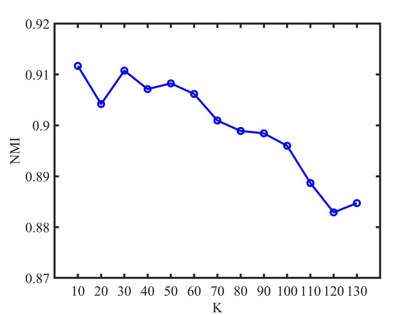
IEEE TRANSACTIONS ON MULTIMEDIA, VOL. XXX, NO. XX, 2021                                                              8

                            TABLE II: ACC(%) results on seven benchmark datasets for all methods
                        Datasets
                                   BBC     BBCSport   3Source     Cora    Handwritten   HW2sources   NGs     MEAN
             Methods
             SCbest                43.94    50.74         39.64   35.82      92.82        58.50      28.96   50.06
             GNMFbest              32.12    32.12         45.56   31.91      73.80        51.10      23.01   41.37
             SCconcat              47.26    67.22         36.45   32.14      60.03        76.24      35.98   50.76
             CCA                   48.12    38.60         41.01   44.15      73.63        74.51      27.62   49.66
             MSE                   39.26    54.01         44.85   31.69      79.84        73.27      27.55   50.07
             MultiNMF              43.36    50.00         52.66   35.60      88.00        76.75      33.61   54.28
             Co-reg                40.73    61.58         45.56   39.11      91.00        82.15      27.45   55.37
             AMGL                  39.21    55.22         42.31   32.05      83.34        90.38      30.83   53.33
             MDcR                  81.05    80.24         70.53   54.51      61.26        86.56      59.06   70.45
             AASC                  38.39    62.32         36.69   33.09      84.65        83.30      71.00   58.49
             WMSC                  42.92    61.21         42.60   42.25      84.50        83.40      43.00   57.12
             AWP                   37.37    44.85         51.48   32.39      96.70        93.85      23.80   54.34
             LRC-MCF               87.45    80.70         78.70   51.18      88.25        99.45      98.20   83.42

                            TABLE III: NMI(%) results on seven benchmark datasets for all methods
                        Datasets
                                   BBC     BBCSport   3Source     Cora    Handwritten   HW2sources   NGs     MEAN
             Methods
             SCbest                23.04    21.20         33.53   16.35      87.78        59.41      7.39    35.53
             GNMFbest              21.43    19.99         29.39   19.14      74.37        57.49      8.85    30.09
             SCconcat              35.45    52.10         35.72   19.22      61.14        80.57      22.75   43.85
             CCA                   30.93    25.30         35.64   26.74      68.15        60.83      13.35   37.28
             MSE                   26.93    34.71         46.61   18.58      80.13        72.17      13.58   41.82
             MultiNMF              27.57    44.69         43.98   26.28      80.25        68.69      20.37   44.55
             Co-reg                23.36    41.22         44.77   22.50      88.33        85.61      7.66    46.21
             AMGL                  26.90    39.92         45.67   18.77      81.08        88.27      19.05   45.67
             MDcR                  61.47    63.94         64.43   31.30      66.65        77.71      50.14   59.34
             AASC                  20.14    39.11         30.21   16.63      87.48        86.14      48.02   46.81
             WMSC                  22.10    47.12         42.00   27.96      87.44        86.50      24.84   48.28
             AWP                   20.06    23.15         41.53   12.26      92.08        91.00      3.88    40.57
             LRC-MCF               73.62    76.00         70.50   37.85      92.03        98.63      93.92   77.50

                           TABLE IV: PUR(%) results on seven benchmark datasets for all methods
                        Datasets
                                   BBC     BBCSport   3Source     Cora    Handwritten   HW2sources   NGs     MEAN
             Methods
             SCbest                49.64    55.70         56.80   40.73      93.29        62.75      29.44   55.48
             GNMFbest              33.43    32.99         56.80   38.40      75.10        59.10      24.88   45.81
             SCconcat              51.42    68.66         55.38   38.43      61.62        79.33      38.86   56.24
             CCA                   52.63    46.47         54.97   50.37      73.69        74.51      29.33   54.57
             MSE                   45.40    56.58         65.56   37.98      80.71        76.96      28.70   55.98
             MultiNMF              43.65    63.42         60.36   49.74      88.00        76.75      35.99   59.70
             Co-reg                49.20    66.91         62.72   45.27      91.00        86.70      28.68   61.50
             AMGL                  45.40    58.93         64.97   38.30      83.34        91.22      32.96   59.30
             MDcR                  81.05    80.24         76.75   56.19      67.22        86.56      69.30   73.90
             AASC                  46.42    67.10         55.03   40.99      87.10        85.85      71.00   64.78
             WMSC                  48.61    68.01         60.36   47.16      87.10        86.10      46.00   63.33
             AWP                   45.69    51.10         63.31   35.60      96.70        93.85      24.40   58.66
             LRC-MCF               87.45    84.38         82.25   52.22      88.05        99.45      98.20   84.57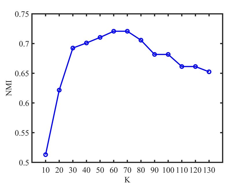
IEEE TRANSACTIONS ON MULTIMEDIA, VOL. XXX, NO. XX, 2021 9
clustering, and shows that LRC-MCF can capture the locality there exists a wide range for each hyper-parameter in which
relationship information and the common similarity relation- relatively stable and good results can be readily obtained.
ships among multiple views. Besides, multi-view methods
cannot always obtain better performance than single-view F. Convergence Analysis
methods, which implies that the diversity and complementary In this section, an iteration updating scheme is adopted by
information cannot be readily exploited. our proposed framework to obtain the optimal solution, thus
For 3Source and Cora datasets, the experimental results convergence analysis is conducted to verify the convergence
show that LRC-MCF can obtain the best performance in terms property of LRC-MCF in detail. We conduct various exper-
of ACC, NMI, and PUR. Besides, most multi-view methods iments on four datasets including BBCSport, Cora, Hand-
outperform single-view methods, which might imply that the written and NGs. Fig. 2 plots the curves of objective values
diversity information among multiple views is benefit for of LRC-MCF with the increase of iterations with respond-
the improvement of clustering performance. However, these ing to the above four datasets. According to the variation
methods cannot get better than RC-MCF, which might be trend of objective values of LRC-MCF in these sub-figures
caused by the issue that the geometric and complementary of Fig.2(a)-Fig.2(d), we can readily find that the objective
information cannot be made full use of. value decreases rapidly during the iterations on all the four
For Handwritten and HW2sources datasets, the experimen- benchmark datasets. Moreover, it’s not difficult to observe
tal results also show that LRC-MCF can performs better than that the convergence can be reached within the 10 steps of
comparing single-view and multi-view clustering methods in iterations. That is to say, LRC-MCF can converge within a
most situations, which can validate the superiority of LRC- limited number of iterations. It also might imply that LRC-
MCF in the domain of image clustering. It implies that the MCF can effectually reduce the redundancy of the learned
locality relationship information in image clustering tasks is representations. However, when facing the complex and large-
the important factor. Thus, how to exploit the common locality scale datasets, it’s necessary to combine it with deep learning
information among multiple views is of great significance. technology [46, 47] to construct the distance function. In the
For NGs dataset, the experimental results show that LRC- future, we consider how to extend superior deep models into
MCF can obtain the best performance in terms of ACC, NMI, our work, which can be optimized by the end-to-end manner.
and PUR. This further validates the effectiveness of LRC-
MCF, which shows that LRC-MCF can fully explore the di-
G. Discussion
versity, geometric, consensus and complementary information
among different views and take sufficient consideration to As the experiment results in Tables II - IV on multi-
weights of different views in finding the common-view locality view clustering tasks, we can clearly find that LRC-MCF
structure. outperforms other comparing methods in most situations. From
Finally, the columns of MEAN in Tables II - IV validate the the above evaluations, it’s readily seen that the embeddings
comprehensive performance of LRC-MCF, the experimental obtained by our method could be more effective and suitable
results show that LRC-MCF can performs better than com- for multi-view features. Besides, other multi-view methods
paring clustering methods in terms of ACC, NMI, and PUR. outperform the other single-view methods in most situations,
It can imply that LRC-MCF not only takes full of the locality which could show multi-view learning is a valuable research
geometric structure and similarity relationship among samples field indeed. Compared to single view methods, taking the
under the multi-view scenario, but explores the diversity, complementary information among different views into con-
consensus and complementary information among different sideration could achieve more excellent performance, and the
views. Thus, LRC-MCF can obtain the best performance on key is how to integrate the complementary information among
seven benchmark datasets in most situations. different views while preserving its intrinsic characteristic in
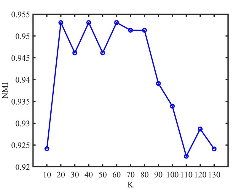
each view. According to Fig. 1, we find that the number K
of nearest neighbors used in our method is relatively smooth
E. Parameter Analysis to the K over the relatively large ranges of values. Note
The proposed LRC-MCF is based on the locality relation- that the experimental results of our proposed LRC-MCF on
ships constraint, thus we need to mainly discuss the sensitivity seven datasets are without fine-tuning, and usage of fine-tuning
analysis on the number K of nearest neighbors used in LRC- might further improve its performance. For the discussion
MCF in this section. Specifically, we conduct the clustering of convergence, according to Fig.2, it could be empirically
experiments for LRC-MCF on BBC, 3Source, HW2sources verified that the proposed LRC-MCF converges once enough
and NGs datasets, then the average value of all evaluation iterations are completed. That is, LRC-MCF could converge
indexes is used as final criteria. Fig. 1 plots the clustering within a limited number of iterations.
results in terms of ACC, NMI, and PUR on these four datasets,
under different K in {10, 20, 30, 40, 50, 60, 70, 80, 90, V. C ONCLUSION
100, 110, 120, 130}. Through these variation trends of ACC, In this paper, we propose a novel multi-view learning
NMI, and PUR over these four datasets, it’s easy to find that method to explore the problem of multi-view clustering,
our method is relatively smooth to the K over the relatively called Locality Relationship Constrained Multi-view Clus-
large ranges of values, which indicates that the performance is tering Framework (LRC-MCF). LRC-MCF attempts to cap-
not so sensitive to those hyper-parameters. More importantly, ture the relationship information among samples under the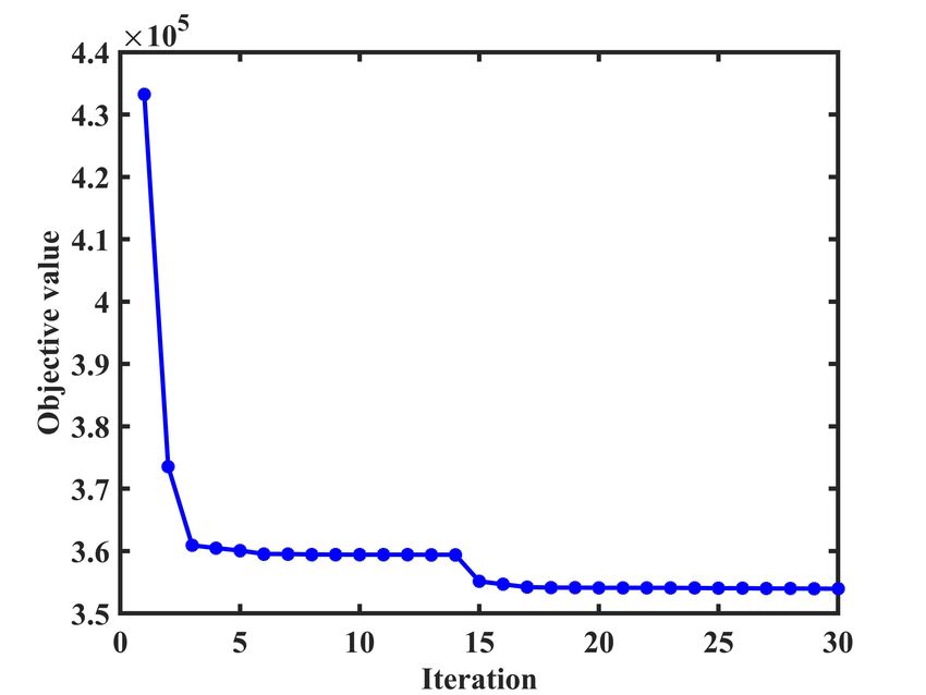
IEEE TRANSACTIONS ON MULTIMEDIA, VOL. XXX, NO. XX, 2021                                                                      10

          (a) ACC in BBC dataset                        (b) NMI in BBC dataset                   (c) PUR in BBC dataset

         (d) ACC in 3Source dataset                    (e) NMI in 3Source dataset            (f) PUR in 3Source dataset

       (g) ACC in Handwritten dataset                (h) NMI in Handwritten dataset         (i) PUR in Handwritten dataset

           (j) ACC in NGs dataset                       (k) NMI in NGs dataset                   (l) PUR in NGs dataset

                                      Fig. 1: K parameter analysis of LRC-MCF on four datasets
IEEE TRANSACTIONS ON MULTIMEDIA, VOL. XXX, NO. XX, 2021 11
(a) BBCSport dataset (b) Cora dataset
(c) Handwritten dataset (d) NGs dataset
Fig. 2: Objective values of LRC-MCF on four datasets
constraint of locality structure and integrate the relationship ACKNOWLEDGMENT
from different views into one common similarity relationships
matrix. Moreover, LRC-MCF provide an adaptive weight The authors would like to thank the anonymous review-
allocation mechanism to take sufficient consideration of the ers for their insightful comments and the suggestions to
importance of different views in finding the common-view significantly improve the quality of this paper. The work
similarity relationships. To effectually reduce the redundancy was supported by the National Natural Science Founda-
of the learned representations, the low-rank constraint on tion of PRChina(72001191), Henan Natural Science Founda-
the common similarity matrix is additionally considered. tion(202300410442), Henan Philosophy and Social Science
Correspondingly, this paper provides an algorithm based on Program(2020CZH009)is gratefully acknowledged. We also
the alternating direction minimization strategy to iteratively would like to thank the anonymous.
calculate all variables of LRC-MCF. Finally, we conduct
extensive experiments on seven benchmark multi-view datasets R EFERENCES
to validate the performance of LRC-MCF, and the experi-
mental results show that the proposed LRC-MCF outperforms [1] C. Zhang, J. Cheng, and Q. Tian, “Multi-view image clas-
its counterparts and achieves comparable performance. In sification with visual, semantic and view consistency,”
the future, we will incorporate our proposed LRC-MCF and IEEE Transactions on Image Processing, vol. 29, pp.
graph-based deep models [48] to further explore multi-view 617–627, 2019.
information in those complex situations. [2] H. Wang, Y. Yang, and B. Liu, “Gmc: Graph-based multi-
view clustering,” IEEE Transactions on Knowledge and
Data Engineering, vol. 32, no. 6, pp. 1116–1129, 2019.
[3] M. R. Amini, N. Usunier, and C. Goutte, “Learning
from multiple partially observed views - an application toIEEE TRANSACTIONS ON MULTIMEDIA, VOL. XXX, NO. XX, 2021 12
multilingual text categorization,” in Advances in Neural [20] L. Tian, F. Nie, and X. Li, “A unified weight learning
Information Processing Systems, 2009, pp. 28–36. paradigm for multi-view learning,” in Proceedings of
[4] G. Bisson and C. Grimal, “Co-clustering of multi-view Machine Learning Research, vol. 89. PMLR, 2019, pp.
datasets: a parallelizable approach,” in International Con- 2790–2800.
ference on Data Mining. IEEE, 2012, pp. 828–833. [21] D. R. Hardoon, S. Szedmak, and J. Shawe-Taylor,
[5] Y. Li, M. Yang, and Z. M. Zhang, “A survey of multi- “Canonical correlation analysis: An overview with ap-
view representation learning,” IEEE Transactions on plication to learning methods,” Neural Computation,
Knowledge and Data Engineering, vol. 31, no. 10, pp. vol. 16, no. 12, pp. 2639–2664, 2004.
1863–1883, 2018. [22] A. Gretton, O. Bousquet, A. Smola, and B. Schölkopf,
[6] H. Zhao and Z. Ding, “Multi-view clustering via deep “Measuring statistical dependence with hilbert-schmidt
matrix factorization,” in AAAI, 2017, pp. 2921–2927. norms,” in International conference on algorithmic learn-
[7] C. Xu, D. Tao, and C. Xu, “Multi-view intact space ing theory. Springer, 2005, pp. 63–77.
learning,” IEEE Transactions on Pattern Analysis and [23] J. Rupnik and J. Shawe-Taylor, “Multi-view canonical
Machine Intelligence, vol. 37, no. 12, pp. 2531–2544, correlation analysis,” in Conference on Data Mining and
2015. Data Warehouses, 2010, pp. 1–4.
[8] M. Kan, S. Shan, and X. Chen, “Multi-view deep network [24] A. Sharma, A. Kumar, H. Daume, and D. W. Jacobs,
for cross-view classification,” in Proceedings of the IEEE “Generalized multiview analysis: A discriminative latent
Conference on Computer Vision and Pattern Recognition, space,” in 2012 IEEE Conference on Computer Vision
2016, pp. 4847–4855. and Pattern Recognition. IEEE, 2012, pp. 2160–2167.
[9] H. Wang, Y. Yang, B. Liu, and H. Fujita, “A [25] M. Kan, S. Shan, H. Zhang, S. Lao, and X. Chen,
study of graph-based system for multi-view clustering,” “Multi-view discriminant analysis,” IEEE Transactions
Knowledge-Based Systems, vol. 163, no. JAN.1, pp. on Pattern Analysis and Machine Intelligence, vol. 38,
1009–1019, 2019. no. 1, pp. 188–194, 2016.
[10] H. Wang, Y. Wang, Z. Zhang, X. Fu, L. Zhuo, M. Xu, [26] Niu, D., Dy, J, Jordan, and a, “Iterative discovery of
and M. Wang, “Kernelized multiview subspace analysis multiple alternativeclustering views,” IEEE Transactions
by self-weighted learning,” IEEE Transactions on Multi- on Pattern Analysis and Machine Intelligence, vol. 36,
media, 2020. no. 7, pp. 1340–1353, 2014.
[11] Z. Zheng, L. Li, F. Shen, S. H. Tao, and S. Ling, “Binary [27] X. Cao, C. Zhang, H. Fu, S. Liu, and H. Zhang,
multi-view clustering,” IEEE Transactions on Pattern “Diversity-induced multi-view subspace clustering,” in
Analysis and Machine Intelligence, vol. 41, no. 7, pp. Computer Vision and Pattern Recognition, 2015, pp.
1774–1782, 2018. 586–594.
[12] Y. Yang and H. Wang, “Multi-view clustering: A survey,” [28] C. Zhang, H. Fu, Q. Hu, P. Zhu, and X. Cao, “Flexible
Big Data Mining and Analytics, vol. 1, no. 2, pp. 83–107, multi-view dimensionality co-reduction,” IEEE Transac-
2018. tions on Image Processing, vol. 26, no. 2, pp. 648–659,
[13] L. Fu, P. Lin, A. V. Vasilakos, and S. Wang, “An overview 2016.
of recent multi-view clustering,” Neurocomputing, vol. [29] W. Wang and Z. H. Zhou, “A new analysis of co-
402, pp. 148–161, 2020. training,” in International Conference on International
[14] Y. Yang and H. Wang, “Multi-view clustering: A survey,” Conference on Machine Learning, 2010.
Big Data Mining and Analytics, vol. 1, no. 2, pp. 83–107, [30] A. Kumar and H. Daumé, “A co-training approach for
2018. multi-view spectral clustering,” in Proceedings of the
[15] G. Chao, S. Sun, and J. Bi, “A survey on multi-view 28th International Conference on Machine Learning,
clustering,” arXiv preprint arXiv:1712.06246, 2017. 2011, pp. 393–400.
[16] T. Xia, D. Tao, T. Mei, and Y. Zhang, “Multiview spectral [31] H. Wang, J. Peng, and X. Fu, “Co-regularized multi-view
embedding,” IEEE Transactions on Systems, Man, and sparse reconstruction embedding for dimension reduc-
Cybernetics, Part B (Cybernetics), vol. 40, no. 6, pp. tion,” Neurocomputing, vol. 347, pp. 191–199, 2019.
1438–1446, 2010. [32] H. Wang, J. Peng, Y. Zhao, and X. Fu, “Multi-path deep
[17] F. Nie, J. Li, and X. Li, “Parameter-free auto-weighted cnns for fine-grained car recognition,” IEEE Transactions
multiple graph learning: A framework for multiview clus- on Vehicular Technology, vol. 69, no. 10, pp. 10 484–
tering and semi-supervised classification,” in Proceedings 10 493, 2020.
of the Twenty-Fifth International Joint Conference on [33] H. Wang, J. Peng, D. Chen, G. Jiang, T. Zhao, and X. Fu,
Artificial Intelligence. AAAI Press, 2016, pp. 181–187. “Attribute-guided feature learning network for vehicle
[18] F. Nie, G. Cai, J. Li, and X. Li, “Auto-weighted multi- reidentification,” IEEE MultiMedia, vol. 27, no. 4, pp.
view learning for image clustering and semi-supervised 112–121, 2020.
classification,” IEEE Transactions on Image Processing, [34] H. Wang, J. Peng, G. Jiang, F. Xu, and X. Fu, “Discrim-
vol. 27, no. 3, pp. 1501–1511, 2017. inative feature and dictionary learning with part-aware
[19] S. Huang, Z. Kang, and Z. Xu, “Self-weighted multi- model for vehicle re-identification,” Neurocomputing,
view clustering with soft capped norm,” Knowledge- 2020.
Based Systems, vol. 158, no. 15, pp. 1–8, 2018. [35] Y. Zhu, Y. Xu, F. Yu, S. Wu, and L. Wang,IEEE TRANSACTIONS ON MULTIMEDIA, VOL. XXX, NO. XX, 2021 13
“Cagnn: Cluster-aware graph neural networks for unsu- Xiangzhu Meng received his B.S. degree from
pervised graph representation learning,” arXiv preprint Anhui University, in 2015, and the Ph.D. degree
in Computer Science and Technology from Dalian
arXiv:2009.01674, 2020. University of Technology, in 2021. Now, he is a
[36] A. Kumar, P. Rai, and H. Daume, “Co-regularized multi- postdoctoral researcher with the Center for Research
view spectral clustering,” in Advances in Neural Infor- on Intelligent Perception and Computing, Institute of
Automation, Chinese Academy of Sciences, China.
mation Processing Systems, 2011, pp. 1413–1421. He regularly publishes papers in prestigious journals,
[37] R. Bhatia, Matrix analysis. Springer Science & Business including Knowledge-Based Systems, Engineering
Media, 2013, vol. 169. Applications of Artificial Intelligence, Neurocom-
puting, etc. In addition, he serves as a reviewer for
[38] V. L. Ulrike, “A tutorial on spectral clustering,” Statistics ACM Transactions on Multimedia Computing Communications and Applica-
and Computing, vol. 17, no. 4, pp. 395–416, 2007. tions. His research interests include multi-modal learning, deep learning, and
[39] D. Cai, X. He, J. Han, and T. S. Huang, “Graph vision-language modeling.
regularized non-negative matrix factorization for data
representation,” IEEE Transactions on Pattern Analysis
and Machine Intelligence, vol. 33, no. 8, pp. 1548–1560,
2011.
[40] J. Liu, C. Wang, J. Gao, and J. Han, “Multi-view
clustering via joint nonnegative matrix factorization,” in
Proceedings of the 2013 SIAM International Conference
on Data Mining. SIAM, 2013, pp. 252–260.
[41] C. Zhang, H. Fu, Q. Hu, P. Zhu, and X. Cao, “Flexible
multi-view dimensionality co-reduction,” IEEE Transac-
tions on Image Processing, pp. 648–659, 2016.
[42] H.-C. Huang, Y.-Y. Chuang, and C.-S. Chen, “Affinity Wei Wei received the B.S. degree from the School
aggregation for spectral clustering,” in 2012 IEEE Con- of Mathematics and Information Science, Henan
University, in 2012, and the Ph.D. degree in Institute
ference on Computer Vision and Pattern Recognition. of Systems Engineering from the Dalian University
IEEE, 2012, pp. 773–780. of Technology, in 2018. He is an associate professor
[43] L. Zong, X. Zhang, X. Liu, and H. Yu, “Weighted multi- of the Center for Energy, Environment & Econ-
omy Research, College of Tourism Management,
view spectral clustering based on spectral perturbation,” Zhengzhou University. His research interests include
in Proceedings of the AAAI Conference on Artificial energy policy analysis, text mining, machine learn-
Intelligence, vol. 32, no. 1, 2018. ing, and artificial intelligence.
[44] F. Nie, L. Tian, and X. Li, “Multiview clustering via
adaptively weighted procrustes,” in Proceedings of the
24th ACM SIGKDD international conference on knowl-
edge discovery & data mining, 2018, pp. 2022–2030.
[45] J. A. Hartigan and M. A. Wong, “A k-means clustering
algorithm,” Applied Statistics, vol. 28, no. 1, 1979.
[46] Y. Zhu, Y. Xu, F. Yu, Q. Liu, S. Wu, and L. Wang,
“Deep graph contrastive representation learning,” in
ICML Workshop on Graph Representation Learning and
Beyond, 2020.
[47] ——, “Graph contrastive learning with adaptive aug-
mentation,” in Proceedings of the Web Conference 2021,
Wenzhe Liu received her BS degree from Qingdao
2021, pp. 2069–2080. University of Science and Technology, in 2013 and
[48] Y. Zhu, W. Xu, J. Zhang, Q. Liu, S. Wu, and L. Wang, received MS degree from Liaoning Normal Univer-
“Deep graph structure learning for robust representations: sity . Now she is working towards the PHD degree in
School of Computer Science and Technology, Dalian
A survey,” arXiv preprint arXiv:2103.03036, 2021. University of Technology, China. Her research inter-
ests include mulit-view learning, deep learning and
data mining.You can also read