Lorentz-violating scenarios in a thermal reservoir
←
→
Page content transcription
If your browser does not render page correctly, please read the page content below
Lorentz-violating scenarios in a thermal reservoir

                                                                                        A. A. Araújo Filho1, ∗
                                                            1
                                                                Universidade Federal do Ceará (UFC), Departamento de Fı́sica,
                                                            Campus do Pici, Fortaleza - CE, C.P. 6030, 60455-760 - Brazil.
                                                                                        (Dated: April 17, 2020)

                                                                                              Abstract
arXiv:2004.07799v1 [hep-th] 16 Apr 2020

                                               In this work, we analyse the thermodynamic properties of the graviton and the generalized
                                          model involving anisotropic Podolsky and Lee-Wick terms with Lorentz violation. We build up
                                          the so-called partition function from the accessible states of the system seeking the following
                                          thermodynamic functions: spectral radiance, mean energy, Helmholtz free energy, entropy and heat
                                          capacity. Besides, we verify that, when the temperature rises, the spectral radiance χ(ν) tends
                                          to attenuate for fixed values of ξ. Notably, when parameter η2 increases, the spectral radiance
                                          χ̄(η2 , ν) weakens until reaching a flat characteristic. Finally, for both theories, we perform the
                                          calculation of the modified black body radiation and the correction to the Stefan–Boltzmann law
                                          in the inflationary era of the universe.

                                          ∗
                                              Electronic address: dilto@fisica.ufc.br

                                                                                                 1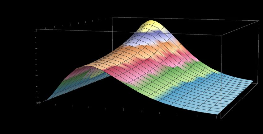
I.    INTRODUCTION

     In theoretical physics, there exists a memorable problem which is putting on an equal
footing the so-called Standard Model [1], provided by a consistent experimental data in pre-
dicting the behavior of fundamental particle physics, and the widespread General Relativity
[2], which has the purpose of regarding gravity as a geometric theory. Since all these ap-
proaches are intensively well tested, if there exists a conciliation for both, one will expect a
unique and fundamental theory of quantum gravity [3]. Moreover, this structure could bring
about the feasibility of investigating some new phenomena not yet individually described by
them. Nevertheless, up to now, there is neither experimental nor observational indications
of any fingerprints of such a unified theory perhaps due to the fact that its effects are high-
lighted when the energy range around the Planck mass, i.e., mP ∼ 1019 GeV, is taken into
account.
     Nowadays, since it is impossible to have the access of such scale, a reasonable way of work-
ing on it has been developed considering the viewpoint that quantum gravity phenomena can
be recognized by the proliferation of their effects at attainable energies. In this sense, one
of the most remarkable possibilities regards the violation of Lorentz symmetry. Supporting
such theory, there are many different mechanisms that bring out Lorentz-violating effects
such as in string theory [4], Horava-Lifshitz gravity [5], noncommutative field theories [6]
and loop quantum gravity [7].
     Having been proposed about thirty years ago by Kostelecký et al., the Standard Model
Extension (SME) [8–12] is an extended version for the usual Standard Model theory. It
possesses Lorentz-violating terms, which are rather tensor terms acquiring a nonzero vacuum
expectation value, coupled with physical fields preserving their coordinate invariance and
a violation of Lorentz symmetry when particle frames are considered [13]. Likewise, such
theoretical background has been the precursor for an expressive number of works involving
the fermionic sector [14–18], the electromagnetic CPT-odd and Lorentz-odd term [19–24] as
well as the CPT-even and Lorentz odd gauge sector [25–28].
     Over the last years, the connection between Lorentz violation and theories including
higher derivative operators has received much attention [29–37]. As a matter of fact, it may
have operators of higher mass dimensions incorporating for instance higher-derivative terms.
Being in contrast to the minimal version of the Lorentz violating extensions, its nonminimal

                                               2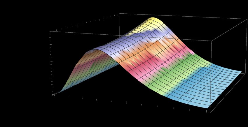
approach has the advantage of possessing an indefinite number of such contributions [32].
In this sense, the latter version of the SME was first proposed considering both the photon
[38] and the fermionic sectors [39].
   In this direction, the first illustration of a higher-derivative electrodynamics was proposed
by Podolsky [40] having a noticeable feature which is the generation of a massive mode
without losing the gauge symmetry. In that paper, it was initially studied the gauge-invariant
dimension-6 term, θ2 ∂α F αβ ∂λ F λβ , with a coupling constant θ, which afterwards would be
known as the Podolsky parameter, with the mass dimension being −1. Clearly, such theory
displays two distinct dispersion relations, i.e., the usual massless mode and the massive mode
which possesses the advantage of avoiding divergences ascribed to the pointlike self-energy.
Nevertheless, considering the quantum level, the latter mode gives rise to the appearance of
ghosts [41].
   Additionally, in the late 1960s, there exists another noteworthy extension of Maxwell
theory with higher derivatives being described by the dimension-6 term Fµν ∂α ∂ α F µν , the
Lee-Wick electrodynamics [42, 43]. Notably, this theory leads to a finite self-energy for
a pointlike charge in (1 + 3) spacetime dimensions and to the appearance of a bilinear
contribution to the Maxwell Lagrangian. This is analogous to the Podolsky term showing
an opposite sign though. Such “incorrect” sign outputs energy instabilities at the classical
level, whereas it brings out a negative norm states in the Hilbert space at the quantum
level. Moreover, it was also Lee and Wick who first proposed a mechanism seeking the
preservation of unitarity by removing all states with negative norm from the Hilbert space.
In the last decade, this theory came back to obtain notability with the proposal of the
Lee-Wick Standard Model [44–46], based on non-Abelian gauge structure free of quadratic
divergences. Such model was widespread having many contributions for both theoretical
and phenomenological approaches [47, 48]. Furthermore, it is worth mentioning that, in this
general context, investigations of Lorentz violation extensions are discussed [49] including
applications to the interaction of pointlike and spatially extended sources [50, 51].
   On the other hand, the focus on an extension of the SME, which takes into account
gravity, arouses from the fact that the Lorentz violation can be expected to be a key element
for a quantum theory of gravitation. As a matter of fact, it is important to note that
Lorentz-violating effects might be expressive in regions where the curvature or torsion are
accentuated, as in the vicinity of black holes for instance [52]. Besides, these implications can

                                              3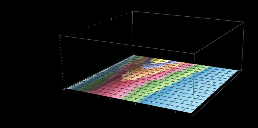
represent a notable role in cosmological scenarios being illustrated by either dark energy [53]
or dark matter [54]. Moreover, there are others whose anisotropy factors can be added in the
Friedman-Robertson-Walker solutions [55]. In addition, the main motivation of constructing
a theory consistent with gravity, i.e., being in agreement with Bianchi identities and so forth,
is having a consistent formalism seeking to maintain the local observer Lorentz covariance,
despite the presence of local particle Lorentz violation [56]. In this way, it is worth pointing
out that there are investigations regarding Lorentz violation in the linearized gravity [57]
and others [58, 59].
      Furthermore, up to now, there are many works based on the analysis of the thermo-
dynamic functions in the gravitational scenario mainly regarding the Cosmic Microwave
Background (CMB) [60–64]. However, there are very few studies of such thermodynamic
properties ascribed to the linearized theory of gravity within the context of Lorentz viola-
tion. In this sense, our starting point is taking into account a similar analysis encountered
in Refs. [60–64], but proposing rather the inflationary epoch of the universe, i.e., 10−13
GeV, within the context of Lorentz violation to utilize the modification from the black body
radiation spectra as well as from the Stefan-Boltzmann law as an alternative to investigate
cosmological scenarios. Besides, for the sake of giving a complement to this analysis, we
provide the calculation of Helmholtz free energy, mean energy, entropy and heat capacity.
      In addition, there is a lack in the literature ascribed to the investigation of the thermo-
dynamic properties for the generalized anisotropic Podolsky with Lee-Wick terms. In this
viewpoint, it is noteworthy to accomplish such analysis in order to verify how the modified
massless mode behaves to perhaps reveal new phenomena which might be applied to either
condensed matter or statistical thermal physics.

II.     GRAVITON WITH LORENTZ VIOLATION

      In this section, we begin with the action responsible for the dynamics of the bumblebee
field Bµ written as
                       ˆ
                              √

                            4      1 µν    2ξ µ ν           µ      2
                SB =       d x −g − B Bµν + 2 B B Rµν − V (B Bµ ∓ b ) ,                      (1)
                                   4       κ

where Bµν = ∂µ Bν − ∂ν Bµ , ξ is a positive parameter which allows the nonminimal coupling
between the bumblebee field and the Ricci tensor Rµν , and κ2 = 32πG is the gravitational

                                                4
coupling constant. Here, it is worth mentioning that, considering the natural units, the
mass dimension of such fields and parameters are [B µ ] = 1, [B µν ] = 2, [κ2 ] = −2, [ξ] = −2.
Next, seeking for simplicity, we adopt the smooth quadratic potential which triggers the
spontaneous Lorentz symmetry breaking
λ 2
V = Bµ B µ ∓ b2 , (2)
2
where the vector bµ is the vacuum expectation value of the bumblebee field Bµ having its
minimum when gµν B µ B ν ±b2 = 0. In Ref. [65], regardless torsion, the authors examined the
graviton spectrum using the weak field approximation for the Einstein-Hilbert gravity in the
context of Lorentz violation. For the sake of obtaining its respective Feynman propagator,
we focus only on the kinetic part
1
Lkin = − hµν Ôµν,αβ hαβ , (3)
2
where Ôµνλσ is the wave operator associated to the theory. Following the definitions en-
countered in Ref. [66], the graviton propagator is defined as follows
h0|T [hµν (x)hαβ (y)]|0i = Dµν,αβ (x − y). (4)
Here, the main issue is finding a closed tensor algebra in order to obtain such operator
Dµν,αβ (x − y) which satisfies the Green’s function
Ôµνλσ Dλσ,αβ (x − y) = iI µν,αβ δ 4 (x − y), (5)
where I µν,αβ plays the role of the identity operator being defined as I µν,αβ = 21 (η µα η νβ +
η µβ η να ). Now, after many algebraic manipulations seeking the inversion of the wave operator
Ôµνλσ , we get
i N1 (1) (2) 1 (0−θ) N4 (0−ω)
Dµν,αβ = 2 2 2
P µν,αβ + P µν,αβ − P µν,αβ + 2 2 2 2
Pµν,αβ
(k) κ ξ (b · k) 2 2λκ ξ (b · k)
2 2
k (2) N5 (0−θω) k (1) N8 (θΣ)
+ Πµν,αβ + 2
P̃µν,αβ + Π̃µν,αβ + Π̃µν,αβ
2ξ(b · k) ξ(b · k) 4ξ(b · k)
√ 2 4
(6)
3k (θΛ) k (ΛΛ) N11 (ωΛ−a)
− Π̃µν,αβ + Π̃µν,αβ + 2 Π̃
2 2 2 8ξ (b · k)2 2 µν,αβ
N12 (ωΛ−b) N13 (ωΣ) N14 (ΛΣ)
+ Π̃ + 2 2 Π̃ + Π̃ ,
2ξ(b · k)2 2 µν,αβ 4κ ξ (b · k)3 2 µν,αβ 4ξ(b · k) 2 µν,αβ
with (k) being given by
(k) = k 2 + ξ(b · k)2 , (7)
5where our attention will be devoted. Moreover, such propagator1 was verified to be physical
reasonable, since it is in agreement with causality and unitarity. Nevertheless, there is no
necessity of working with the full expression in our case, since all we need is fully contained
in the pole of the propagator, i.e., (k). In possession of this, the following calculations will
be performed in order to derive all the main thermodynamic functions. For doing so, we
proceed further seeking the number of the available states of the system in order to build up
the so-called partition function. Here, we start with the following dispersion relation given
by
k 2 + ξ(b · k)2 = 0,
and, in this sense, we invoke the accessible states of the system written as
ˆ ∞
Γ
Ω(ξ) = 2 (1 + ξ)3/2 E 2 dE, (8)
π 0
where Γ is the volume of the thermal reservoir. Now, let us remind here that the link between
the thermal behavior and the macroscopic world is carried out by the partition function.
Then, we are properly able to write it down
ˆ ∞
Γ
(1 + ξ)3/2 E 2 ln 1 − e−βE dE,
ln [Z(β, Γ)] = − 2 (9)
π 0
where β = 1/κB T and T is the temperature of the Universe. The above expression is
similar to Bose-Einstein statistics but rather having a modification due to parameter ξ. In
a straightforward manner, using the advantage of taking into account Eq.(9), we can obtain
the thermodynamic functions per volume Γ, namely, the Helmholtz free energy F (β, ξ), the
mean energy U (β, ξ), the entropy S(β, ξ) and the heat capacity CV (β, ξ), defined as follows:
1
F (β, ξ) = − ln [Z(β, ξ)] ,
β
∂
U (β, ξ) = − ln [Z(β, ξ)] ,
∂β
(10)
∂
S(β, ξ) = kB β 2 F (β, ξ),
∂β
∂
CV (β, ξ) = −kB β 2 U (β, ξ).
∂β
1
If one is interested in any missing definitions of Eq. (6), see Ref. [65] for further details.
6At the beginning, let us consider the mean energy
ˆ ∞
1 (1 + ξ)3/2 E 3 e−βE
U (β, ξ) = 2 dE, (11)
π 0 (1 − e−βE )
which follows the spectral radiance given by:
(hν)3 (1 + ξ)3/2 e−βhν
χ(ξ, ν) = , (12)
π 2 (1 − e−βhν )
where we have regarded E = hν, as h being the Planck constant and ν the frequency.
The plot of the above equation is exhibited in Fig. 1 concerning three different cases when
parameters ξ and β vary. This and other comments are better explained and discussed
in Section IV. Looking towards to recover the radiation constant of the Stefan-Boltzmann
ξ=1 1.4 × 1039 ξ=1, β=1.5x10⁻¹³
3.0 × 1040
ξ=3 1.2 × 1039
2.5 × 1040 ξ=3, β=2x10-13
ξ=5 1.0 × 1039
2.0 × 1040 ξ=5, β=2.5x10⁻¹³
ξ=7 8.0 × 1038
χ(ν)
χ(ν)
1.5 × 1040 ξ=7, β=3.5x10⁻¹³
6.0 × 1038
1.0 × 1040 ξ=10, β=5x10-13
4.0 × 1038
5.0 × 1039 2.0 × 1038
0 0
0 2 × 10¹³ 4 × 10¹³ 6 × 10¹³ 8 × 10¹³ 1 × 10¹⁴ 0 2 × 10¹³ 4 × 10¹³ 6 × 10¹³ 8 × 10¹³ 1 × 10¹⁴
ν ν
1.2 × 1039
β= 1.5x10⁻¹³
1.0 × 1039 β= 2x10-13
8.0 × 1038 β= 2.5x10⁻¹³
χ(ν)
6.0 × 1038 β= 3.5x10⁻¹³
4.0 × 1038
2.0 × 1038
0
0 2 × 10¹³ 4 × 10¹³ 6 × 10¹³ 8 × 10¹³ 1 × 10¹⁴
ν
Figure 1: The plots exhibit how the spectral radiance χ(ν) changes as a function of frequency ν
for different scenarios with h = 1.
energy, i.e., uS = αT 4 , we consider ξ −→ 0 leading to
ˆ ∞
1 E 3 e−βE π2
α= 2 dE = , (13)
π 0 (1 − e−βE ) 15
which reproduces the well-established result in the literature [67]. Now, for the sake of
completeness, it is important to point out that hereafter, unless stated otherwise, all the
7following computations will be performed having the temperature β = 10−13 GeV, κB = 1,
as well as the density per volume Γ approach. In this sense, in order to check how the
coupling constant ξ affects the new radiation constant and all the remaining thermodynamic
functions, we proceed as follows:
α̃ ≡ U (β, ξ)β 4 , (14)
and we calculate the Helmholtz free energy
ˆ ∞
1
(1 + ξ)3/2 E 2 ln 1 − e−βE dE,
F (β, ξ) = 2 (15)
π β 0
the entropy
ˆ ∞ ˆ ∞
(1 + ξ)3/2 E 3 e−βE
κB 3/2 2 −βE
S(β, ξ) = 2 − (1 + ξ) E ln 1 − e +β dE, (16)
π 0 0 1 − e−βE
and the heat capacity
ˆ ∞ ˆ ∞
κB β 2 (1 + ξ)3/2 E 4 e−2βE (1 + ξ)3/2 E 4 e−βE
CV (β, ξ) = + dE. (17)
π2 0 (1 − e−βE )2 0 1 − e−βE
Now, having obtained these expressions, we can solve them numerically and their following
results are displayed in Fig. 2. Notably, within the context of a linearized theory of gravity,
there exists a corresponding intrinsic entropy ascribed to any distribution of gravitational
radiation [68] and a well-behavior conjecture having the absence of an ultraviolet catastrophe
[69].
III. GENERALIZED MODEL WITH PODOLSKY AND LEE-WICK TERMS
Recently, in the literature, the authors proposed an effective model of higher-derivative
electrodynamics in the context of Lorentz violation which studies some classical aspects
regarding unitarity and causality from the propagator, i.e., it is proposed a generalized
model involving anisotropic Podolsky and Lee-Wick terms [34]. In such reference, it is used
the advantage of regarding the spin-projection operators [70, 71], seeking a closed algebra
in order to calculate the propagator of this respective theory. For doing so, the prescription
of a rank-2 symmetric tensor Dβα = (Bβ Cα − Bα Cβ )/2 (where Bβ and Cα are constant
four-vectors which account for Lorentz violation) has been invoked. In this sense, it was
considered a more general dimension-6 higher-derivative Lagrangian
1 θ2 1
L = − F µν Fµν + ∂α F αβ ∂λ F λβ + η12 Dβα ∂σ F σβ ∂λ F λα + η22 Dβα ∂σ F σλ ∂β Fαλ + (∂µ Aµ )2
4 2 2ξ˜
(18)
86000 8 × 1042
5000
6 × 1042
4000
S(ξ)
˜(ξ)
3000 4 × 1042
α
2000
2 × 1042
1000
0 0
0 20 40 60 80 100 0 20 40 60 80 100
ξ ξ
0 2.5 × 1043
-5.0 × 1041 2.0 × 1043
-1.0 × 1042 1.5 × 1043
C V (ξ)
F(ξ)
1.0 × 1043
-1.5 × 1042
5.0 × 1042
-2.0 × 1042
0
0 20 40 60 80 100 0 20 40 60 80 100
ξ ξ
Figure 2: The figure shows the correction to the so-called Stefan–Boltzmann law represented by
parameter α̃(ξ), the entropy S(ξ), the Helmholtz free energy F (ξ) and the heat capacity CV (ξ),
considering κB = 1 in the high temperature regime of the universe, namely, β = 10−13 GeV.
where θ, η1 and η2 are coupling constants with positive defined values and ξ˜ is the gauge
fixing parameter to invert the wave operator associated with the Lagrangian of this theory.
Besides, Eq. (18) leads to the corresponding propagator2
i ˜
Ξ̃να (k) = − 2
{Γ̃(k)Θνα + [b0 − ξ∆(k)]Ωνα − iF̃ (k)(Bν kα + Bα kν )
k ∆(k)
− 2η12 Dνα k 2 Π̃(k) − iH̃(k)(Cν kα + Cα kν ) (19)
+ η14 Bν Bα [(C · k)2 − C 2 k 2 ]k 2 + η14 Cν Cα [(B · k)2 − B 2 k 2 ]k 2 },
where Γ̃(k) = η14 [(B · k)2 − B 2 k 2 ][(C · k)2 − C 2 k 2 ] − {1 − θ2 k 2 − η12 k 2 (B · C) + [η12 − 2η22 ]
× (B · k)(C · k)}2 and ∆(k) = 1 − θ2 k 2 − η22 (B · k)(C · k) Γ̃(k). In addition, Eq. (18) gives
rise to the following dispersion relation
h i
k 2 1 − θ2 k 2 − η22 (B · k)(C · k) Γ̃(k) = 0. (20)
2
Likewise in the previous section, for any missing definitions of Eq. (19), see Ref.[34] for further details.
9Here, let us regard the timelike isotropic sector, namely, Bµ = (B0 , 0) and Cµ = (C0 , 0),
which follows the bottom expression
θ2 1
E2 = 2
k2 + 2 , (21)
2
θ + 2η2 B0 C0 θ + 2η22 B0 C0
where, notably, the term θ2 /(θ2 +2η22 B0 C0 ) may be identified as a dielectric constant modify-
ing the usual Podolsky electrodynamics. In possession of Eq. (21) and considering a photon
gas in a thermal bath, the number of available states can be derived in a straightforward
way:
ˆ ∞ −3/2 s
θ2
1 1
Ω̄(θ, η2 , B0 , C0 ) = 2 E E2 − dE, (22)
π 0 θ2 + 2η22 B0 C0 θ2 + 2η22 B0 C0
yielding the partition function, which may be properly written as
ˆ ∞ −3/2 s
1 θ2 2−
1 βE
ln[Z̄(θ, β, η2 , B0 , C0 )] = − 2 E E ln 1 − e dE.
π 0 θ2 + 2η22 B0 C0 θ2 + 2η22 B0 C0
(23)
Additionally, it is important to mention that in different contexts, many works have been
made in such direction [35, 72–74] and a Podolsky term can be generated if quantum correc-
tions are taken into account regarding a condensation of topological defects [75]. Here, from
Eq. (23), an analogous process to calculate all those thermodynamic quantities presented
in the previous section can be performed as well. In this way, we have the mean energy
ˆ ∞ 2
−3/2 s −βE
1 2 θ 2
1 e
Ū (θ, β, η2 , B0 , C0 ) = 2 E 2
E − 2 2
dE,
π 0 2
θ + 2η2 B0 C0 θ + 2η2 B0 C0 1 − e−βE
(24)
which follows the spectral radiance
−3/2 s
θ2 e−βE
1 1
χ̄(θ, β, η2 , B0 , C0 ) = 2 E 2 E2 − , (25)
π θ2 + 2η22 B0 C0 θ + 2η22 B0 C0
2 1 − e−βE
plotted in Fig. 3 for different values of η2 . Again, the same procedure of inferring how the
new radiation constant of the Stefan–Boltzmann law behaves, namely ᾱ(θ, β, η2 , B0 , C0 ), is
performed as well in what follows. Next, we derive all the remaining ones: the Helmholtz
free energy
ˆ ∞ −3/2 s
θ2
1 1
ln 1 − eβE dE,
F̄ (θ, β, η2 , B0 , C0 ) = 2 2 E E2 −
β π 0 θ2 + 2η22 B0 C0 θ2 2
+ 2η2 B0 C0
(26)
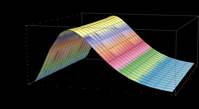
10Figure 3: This figure shows the behavior of the spectral radiance χ̄(ν) for different values of η2 and
ν. We consider fixed values of B0 , C0 and θ, i.e., B0 = C0 = 1 and θ = 10, in the context of the
temperature in the inflationary era of the universe, i.e., β = 10−13 GeV.
the entropy
ˆ ∞ −3/2 s
θ2
1 2−
1 −βE
S̄(θ, β, η2 , B0 , C0 ) = − 2 E 2
E 2
ln 1 − e dE
π0 θ2 + 2η2 B0 C0 θ2 + 2η2 B0 C0
ˆ ∞ 2
−3/2 s −βE
β 2 θ 2−
1 e
+ 2 E 2
E 2
dE,
π 0 θ2 + 2η2 B0 C0 θ2 + 2η2 B0 C0 1 − e−βE
(27)
and, finally, the heat capacity
ˆ ∞ −3/2 s
β2 θ2 e−2βE
3 1
C̄V (θ, β, η2 , B0 , C0 ) = + 2 E E2 − dE
π0 θ2 + 2η22 B0 C0 (1 − e−βE )2
θ + 2η22 B0 C0
2
ˆ −3/2 s
β2 ∞ 3
−βE
θ2
2
1 e
+ 2 E 2
E − 2 2
dE.
π 0 2
θ + 2η2 B0 C0 θ + 2η2 B0 C0 1 − e−βE
(28)
Furthermore, the graphics of these quantities are displayed in Fig. 4. It is worth mentioning
that even though there exists the appearance of a minus sign in all those square roots, as
long as the positive defined values of θ and η2 are considered, the theory does not possess
11any disturbing issues ascribed to imaginary energies. In addition, considering also the CPT-
even scenario, the authors calculated the contribution to the free energy in the rotationally
invariant Lorentz-violating quantum electrodynamics as well as the correction to the pressure
for one-and two-loop approximations at high temperature regime [76].
8 × 1040
8 × 10¹⁷
6 × 1040
6 × 10¹⁷
α(η2 )
S(η2 )
4 × 1040
4 × 10¹⁷
2 × 10¹⁷ 2 × 1040
0 0
0 2 × 10⁶ 4 × 10⁶ 6 × 10⁶ 8 × 10⁶ 1 × 10⁷ 0 200 400 600 800 1000
η2 η2
0 2.5 × 1041
2.0 × 1041
-5.0 × 1065
1.5 × 1041
C V (η2 )
F(η2 )
-1.0 × 1066
1.0 × 1041
-1.5 × 1066
5.0 × 1040
-2.0 × 1066
0
0 200 400 600 800 1000 0 200 400 600 800 1000
η2 η2
Figure 4: The figure displays the correction to the so-called Stefan–Boltzmann law represented by
parameter ᾱ(η2 ), the entropy S̄(η2 ), the Helmholtz free energy F̄ (η2 ) and the heat capacity C̄V (η2 )
considering κB = 1 in the inflationary epoch of the universe, i.e., β = 10−13 GeV.
IV. RESULTS AND DISCUSSIONS
At the beginning, we started off with the subsequent discussion regarding the thermo-
dynamic aspects of the graviton with Lorentz violation. In this sense, we proceeded the
calculations seeking the number of available states of the system which came from the given
dispersion relation exhibited in Eq. (7). From it, the so-called partition function was built
up in Eq. (9) which sufficed to provide all the required thermodynamic functions, i.e., the
spectral radiance χ(β, ξ), the mean energy U (β, ξ), the Helmholtz free energy F (β, ξ), the
entropy S(β, ξ) and the heat capacity CV (β, ξ).
12Next, in Fig 1, the spectral radiance was plotted for three different cases, namely, on the
top left, the graphic exhibited how χ(ν) changed as a function of ν for a fixed temperature
β = 10−13 GeV; on the top right, it was shown how χ(ν) evolved for diverse values of ξ
and β; on the other hand, on the bottom one, the plot presented the behavior of χ(ν) for
distinct temperatures considering ξ = 1. Besides, in Fig 2, it was displayed the modification
to the Stefan–Boltzmann law represented by parameter α̃(ξ) exhibiting the characteristic
of a monotonically increasing function. The same behavior was also presented when one
considered the entropy S(β, ξ) and the heat capacity CV (β, ξ). However, having a different
behavior from the other ones, the Helmholtz free energy F (β, ξ) showed a monotonically
decreasing function when ξ started to increase.
Now, let us take into account the theory of generalized Podolsky with Lee-Wick terms.
Likewise, we calculated the same thermodynamic functions for this case. In Fig. 3, it was
displayed how the spectral radiance evolved when η2 and ν changed for fixed values of β, B0 ,
C0 and θ, i.e., β = 10−13 GeV, B0 = C0 = 1 and θ = 10 respectively. In such direction, it is
worth mentioning that there was an intriguing point due to the fact that when one considered
η2 > 5, one obtained a sudden behavior of such plot, namely, the flatness characteristic of
the spectral radiance χ̄(η2 , ν).
Furthermore, in Fig. 4, the correction to the Stefan–Boltzmann law characterized by ᾱ(η2 )
was shown to have an expressive positive curvature of such curve for huge values of η2 . This
differed from the analysis accomplished by the study of the graviton modified by Lorentz
violation, since the latter showed a very smooth curvature. Now, considering both the
entropy S̄(η2 ) and the heat capacity C̄V (η2 ), we verified that they presented a monotonically
increasing function with a very smooth curvature when η2 changed, being similar to those
aspects concerning the study of the thermodynamic properties of the graviton in the context
of Lorentz violation. Finally, having an analogous behavior of such theory, the Helmholtz
free energy F̄ (η2 ) showed a monotonically decreasing curve when η2 changed.
13V. CONCLUSION
This work focused on investigating the thermodynamic properties of the graviton and a
modified photon gas, which came from a generalized electrodynamics including anisotropic
Podolsky and Lee-Wick terms, in a thermal reservoir when Lorentz violation is taken into
account. In this direction, we determined the number of accessible states of the system which
played a crucial role in obtaining the partition function. It sufficed to supply all the main
thermodynamic functions, namely, spectral radiance, mean energy, Helmholtz free energy,
entropy and heat capacity. Again, it is important to be noticed that the entire study was
performed dealing with a high temperature regime, i.e., β = 10−13 GeV. Additionally, we
proposed a correction to the black body radiation spectra as well as to the Stefan–Boltzmann
law in terms of ξ and η2 .
Next, in the context of graviton thermodynamics with Lorentz violation, the parameter
α̃(ξ) expressed the particular feature of being a monotonically increasing function. The same
property was also displayed when one regarded the entropy S(β, ξ) and the heat capacity
CV (β, ξ). In contrast, being the distinct one, the Helmholtz free energy F (β, ξ) indicated a
monotonically decreasing function when parameter ξ increased.
On the other hand, considering the generalized Podolsky with addition of Lee-Wick terms,
ᾱ(η2 ) possessed a significant positive curvature for huge values of η2 . Notably, taking into
account the entropy S̄(η2 ) and the heat capacity C̄V (η2 ), one verified that such plots had a
monotonically increasing function with an attenuated curvature. In a complementary way,
the Helmholtz free energy F̄ (η2 ) showed a monotonically decreasing curve.
Lastly, the physical implications of the thermodynamic properties presented by the gravi-
ton might address some new fingerprints of a hidden physics which might be confronted with
observatory data in the existence of Lorentz violation. In such direction, these proposals can
address a toy model for further studies involving gravitation and cosmology. Besides, with
respect to the generalized theory of Podolsky with Lee-Wick terms, these properties might
be advantageous in either forthcoming approaches regarding condensed matter physics or
statistical thermodynamics. As a future perspective, examining the thermal features of very
recent models, which appeared in the literature involving the Stückelberg electrodynamics
modified by a Carroll-Field-Jackiw term [77], and the graviton-dark photons in cosmological
scenarios [78], seem to be interesting open questions to be investigated.
14Acknowledgments
The author would like to thank the Conselho Nacional de Desenvolvimento Cientı́fico
e Tecnológico (CNPq) for the financial support, L.L. Mesquita for the careful reading of
this manuscript and A.Y. Petrov for the fruitful discussions and suggestions during the
preparation of this work.
[1] M. D. Schwartz, Quantum field theory and the standard model (Cambridge University Press,
2014).
[2] R. M. Wald, General relativity (University of Chicago press, 2010).
[3] C. Rovelli, Quantum gravity (Cambridge university press, 2004).
[4] N. E. Mavromatos, arXiv preprint arXiv:0708.2250 (2007).
[5] M. Pospelov and Y. Shang, Physical Review D 85, 105001 (2012).
[6] S. M. Carroll, J. A. Harvey, V. A. Kosteleckỳ, C. D. Lane, and T. Okamoto, Physical Review
Letters 87, 141601 (2001).
[7] J. Alfaro, H. A. Morales-Tecotl, and L. F. Urrutia, Physical Review D 65, 103509 (2002).
[8] D. Colladay and V. A. Kosteleckỳ, Physical Review D 58, 116002 (1998).
[9] D. Colladay and V. A. Kosteleckỳ, Physical Review D 58, 116002 (1998).
[10] V. A. Kosteleckỳ and S. Samuel, Physical Review Letters 63, 224 (1989).
[11] V. A. Kosteleckỳ and S. Samuel, Physical Review D 39, 683 (1989).
[12] V. A. Kosteleckỳ and R. Potting, Physics Letters B 381, 89 (1996).
[13] V. A. Kosteleckỳ and R. Lehnert, Physical Review D 63, 065008 (2001).
[14] G. M. Shore, Nuclear Physics B 717, 86 (2005).
[15] D. Colladay and V. A. Kosteleckỳ, Physics Letters B 511, 209 (2001).
[16] O. Kharlanov and V. C. Zhukovsky, Journal of mathematical physics 48, 092302 (2007).
[17] R. Bluhm, V. A. Kosteleckỳ, and C. D. Lane, Physical Review Letters 84, 1098 (2000).
[18] S. Kruglov, Physics Letters B 718, 228 (2012).
[19] C. Adam and F. R. Klinkhamer, Nuclear Physics B 607, 247 (2001).
[20] A. A. Andrianov and R. Soldati, Physics Letters B 435, 449 (1998).
[21] A. A. Andrianov, R. Soldati, and L. Sorbo, Physical Review D 59, 025002 (1998).
15[22] H. Belich, L. Bernald, P. Gaete, and J. Helayël-Neto, The European Physical Journal C 73,
2632 (2013).
[23] A. B. Scarpelli, H. Belich, J. Boldo, and J. Helayel-Neto, Physical Review D 67, 085021
(2003).
[24] J. Alfaro, A. Andrianov, M. Cambiaso, P. Giacconi, and R. Soldati, International Journal of
Modern Physics A 25, 3271 (2010).
[25] V. A. Kosteleckỳ and M. Mewes, Physical Review Letters 87, 251304 (2001).
[26] F. Klinkhamer and M. Risse, Physical Review D 77, 016002 (2008).
[27] B. Altschul, Physical review letters 98, 041603 (2007).
[28] M. Schreck, Physical Review D 86, 065038 (2012).
[29] R. Casana, M. Ferreira Jr, E. Passos, F. dos Santos, and E. Silva, Physical Review D 87,
047701 (2013).
[30] R. Casana, M. Ferreira Jr, R. Maluf, and F. dos Santos, Physics Letters B 726, 815 (2013).
[31] H. Belich, L. Colatto, T. Costa-Soares, J. Helayël-Neto, and M. Orlando, The European
Physical Journal C 62, 425 (2009).
[32] M. Schreck, Physical Review D 90, 085025 (2014).
[33] R. Cuzinatto, C. De Melo, L. Medeiros, and P. Pompeia, International Journal of Modern
Physics A 26, 3641 (2011).
[34] R. Casana, M. M. Ferreira Jr, L. Lisboa-Santos, F. E. dos Santos, and M. Schreck, Physical
Review D 97, 115043 (2018).
[35] A. A. Filho and R. Maluf, arXiv preprint arXiv:2003.02380 (2020).
[36] M. Anacleto, F. Brito, E. Maciel, A. Mohammadi, E. Passos, W. Santos, and J. Santos,
Physics Letters B 785, 191 (2018).
[37] L. Borges, F. Barone, C. de Melo, and F. Barone, Nuclear Physics B 944, 114634 (2019).
[38] V. A. Kosteleckỳ and M. Mewes, Physical Review D 80, 015020 (2009).
[39] V. A. Kosteleckỳ and M. Mewes, Physical Review D 88, 096006 (2013).
[40] B. Podolsky, Physical Review 62, 68 (1942).
[41] A. Accioly and E. Scatena, Modern Physics Letters A 25, 269 (2010).
[42] T. Lee and G. Wick, Nuclear Physics B 9, 209 (1969).
[43] T. Lee and G. Wick, Physical Review D 2, 1033 (1970).
[44] R. S. Chivukula, A. Farzinnia, R. Foadi, and E. H. Simmons, Physical Review D 82, 035015
16(2010).
[45] T. E. Underwood and R. Zwicky, Physical Review D 79, 035016 (2009).
[46] B. Grinstein and D. O’Connell, Physical Review D 78, 105005 (2008).
[47] C. D. Carone and R. F. Lebed, Journal of High Energy Physics 2009, 043 (2009).
[48] E. Alvarez, L. Da Rold, C. Schat, and A. Szynkman, Journal of High Energy Physics 2009,
023 (2009).
[49] R. Turcati and M. Neves, Advances in High Energy Physics 2014 (2014).
[50] A. Accioly, J. Helayël-Neto, F. Barone, F. Barone, and P. Gaete, Physical Review D 90,
105029 (2014).
[51] F. Barone, G. Flores-Hidalgo, and A. Nogueira, Physical Review D 91, 027701 (2015).
[52] E. Barausse and T. P. Sotiriou, Classical and Quantum Gravity 30, 244010 (2013).
[53] P. J. E. Peebles and B. Ratra, Reviews of modern physics 75, 559 (2003).
[54] N. Arkani-Hamed, D. P. Finkbeiner, T. R. Slatyer, and N. Weiner, Physical Review D 79,
015014 (2009).
[55] S. W. Hawking and G. F. R. Ellis, The large scale structure of space-time, Vol. 1 (Cambridge
university press, 1973).
[56] V. A. Kosteleckỳ, Physical Review D 69, 105009 (2004).
[57] A. Ferrari, M. Gomes, J. Nascimento, E. Passos, A. Y. Petrov, and A. da Silva, Physics
Letters B 652, 174 (2007).
[58] J. Boldo, J. Helayel-Neto, L. De Moraes, C. Sasaki, and V. V. Otoya, Physics Letters B 689,
112 (2010).
[59] B. Pereira-Dias, C. Hernaski, and J. Helayël-Neto, Physical Review D 83, 084011 (2011).
[60] J. C. Magueijo, Physical Review D 49, 671 (1994).
[61] A. N. Cillis and D. D. Harari, Physical Review D 54, 4757 (1996).
[62] P. Chen, Physical review letters 74, 634 (1995).
[63] D. Ejlli, Physical Review D 87, 124029 (2013).
[64] P. Chen and T. Suyama, Physical Review D 88, 123521 (2013).
[65] R. Maluf, C. Almeida, R. Casana, and M. Ferreira Jr, Physical Review D 90, 025007 (2014).
[66] R. Maluf, V. Santos, W. Cruz, and C. Almeida, Physical Review D 88, 025005 (2013).
[67] F. Reif, Fundamentals of statistical and thermal physics (Waveland Press, 2009).
[68] L. Smolin, General relativity and gravitation 17, 417 (1985).
17[69] L. Smolin, General relativity and gravitation 16, 205 (1984).
[70] A. B. Scarpelli, H. Belich, J. Boldo, and J. Helayel-Neto, Physical Review D 67, 085021
(2003).
[71] R. Maluf, A. Araújo Filho, W. Cruz, and C. Almeida, EPL (Europhysics Letters) 124, 61001
(2019).
[72] M. Pacheco, R. Maluf, C. Almeida, and R. Landim, EPL (Europhysics Letters) 108, 10005
(2014).
[73] R. R. Oliveira, A. A. Araújo Filho, F. C. Lima, R. V. Maluf, and C. A. Almeida, The
European Physical Journal Plus 134, 495 (2019).
[74] R. Oliveira and A. Araújo Filho, The European Physical Journal Plus 135, 99 (2020).
[75] D. Granado, A. Carvalho, A. Y. Petrov, and P. Porfirio, arXiv preprint arXiv:1912.00855
(2019).
[76] M. Gomes, T. Mariz, J. Nascimento, A. Y. Petrov, A. Santos, and A. da Silva, Physical
Review D 81, 045013 (2010).
[77] M. M. Ferreira Jr, J. A. Helayël-Neto, C. M. Reyes, M. Schreck, and P. D. Silva, Physics
Letters B , 135379 (2020).
[78] E. Masaki and J. Soda, Physical Review D 98, 023540 (2018).
18You can also read