Many Losers and A Few Winners: The Impact of COVID-19 on Canadian Industries and Regions
←
→
Page content transcription
If your browser does not render page correctly, please read the page content below
Many Losers and A Few Winners:
   The Impact of COVID–19 on Canadian
          Industries and Regions
                               Margaret E. Slade
                       The Vancouver School of Economics

Abstract. COVID–19 has affected all industrial sectors and regions of the world
and, in many cases, the impact has been devastating. Nevertheless, there are large
differences across sectors and regions, with a few winners as well as many losers. This
paper assesses the impact of the first wave of the virus on Canadian industries and
provinces in the short and medium run. In particular, time–series forecasting models
for 39 three–digit industries in each of the ten provinces are estimated and used to
predict post–lockdown losses: percentage differences between forecast and observed
economic activity. Econometric analysis of the estimates is then used to quantify
and rank industries and provinces in terms of short and medium term losses and
gains. Provincial ranks are then compared to the stringency of provincial economic
restrictions.

Résumé. If you do not provide a French abstract, the English abstract will be
translated into French and inserted here.

JEL classification: C22, C53, R11

1. Introduction
COVID–19, which has affected all aspects of economic activity, is the
largest shock to hit the world economy since World War II. Furthermore,
since outbreaks of this magnitude are extremely rare and unprecedented in
the preceding 100 years, the consequences were difficult if not impossible
to predict. Not surprisingly, governments and regions were completely

   I would like to thank Joris Pinkse, Nancy Gallini, the editor Hashmat Kahn, and two
   anonymous referees for helpful suggestions. I would also like to thank Charles Breton
   for allowing me to use his data on provincial restrictions.
   Corresponding author: Margret E. Slade, mslade@mail.ubc.ca

Canadian Journal of Economics / Revue canadienne d’économique 20XX 00(0)
January 20XX. Printed in Canada / Janvier 20XX. Imprimé au Canada

ISSN: 0000-0000 / 20XX / pp. 1–?? / © Canadian Economics Association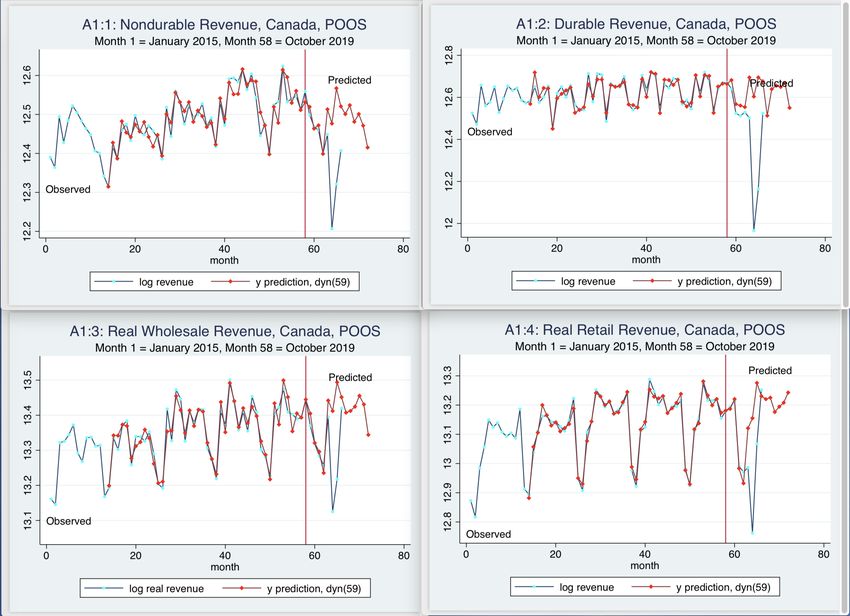
2   Margaret E. Slade

unprepared for a calamity of that magnitude and the reductions in output
that ensued.
   The virus has generated an outpouring of academic research that examines
economic topics such as: health and epidemiology;1 , jobs and unemployment;
poverty, inequality, and income distribution; minorities and race; taxes,
subsidies, and public policy; GDP growth and development; movement of
goods and people across borders; stock market reactions; small business
survival; and environmental consequences. However, little has been written
about how the virus has affected individual industries in different regions.2
   This paper examines the impact of the first wave of COVID–19 on 39 three–
digit industries in each of the ten Canadian provinces in both the short and
medium run. Specifically, for each industry and province pair, I estimate a
time–series forecasting model that is used to predict post–lockdown output.
The forecasts are then compared to realized output. In particular, percentage
differences between realized and forecast output are calculated for the first
month of the lockdown (March) and are also averaged over a four–month
period (March–June). Econometric analysis of the individual estimates is then
used to quantify and rank industries and provinces in terms of short and
medium term losses and gains.
   Although absence from work due to sickness was a factor in determining
economic losses, provincial responses to the virus in the form of mandated
closures and restrictions on other activity such as travel, which occurred early
on and were severe, are likely to have had much larger economic consequences.
Furthermore, although the provinces adopted similar responses at similar
times – for example, all declared states of emergencies within a 9–day period —
there were provincial differences in both the severity of the measures adopted
and the timing of their adoption. I examine whether those differences can
explain variation in the estimated output losses.
   The first wave of the pandemic was different from the second in several
respects. In particular, responses in the form of closures and restrictions were
much more severe and came much sooner. This was probably due to the
fact that so little was known about the virus in the first few months and a
conservative approach was considered prudent. In addition, the recovery was
much swifter. These facts mean that the first wave is a well defined episode.
   A common method of assessing the health of markets is to compare current
outcomes to outcomes in the previous month and in the same month of the

1 Health and epidemiology is perhaps the largest category. Examples in the Canadian
  context include Aguirregabiria et al. (2020), Brodeur et al. (2020), Casares and Khan
  (2020), and Mohammed et al. (2020), who examine the spread of the virus and evaluate
  the effect of the public policies that were adopted. The effect of the virus on the
  Canadian labour market is assessed in Jones et al. (2020), Lemieux et al. (2020), and
  Qian and Fulller (2020).
2 A number of papers examine the effects of the virus on small businesses in the US, e.g.,
  Bartik et al. (2020) and Fairlie (2020).

Canadian Journal of Economics / Revue canadienne d’économique 20XX 00(0)
Many Losers and a Few Winners        3

previous year. For example, a Vancouver realtor’s web page states that “There
were 3,684 homes newly listed on the Multiple Listing Service (MLS) system
in Metro Vancouver in May 2020. This number represents a 37.1% decrease
compared to May 2019, and a 59.3% increase compared to April 2020.”3
However, from a forecasting point of view, month–to–month comparisons
are flawed because most economic activity is highly seasonal, and year–to–
year comparisons are flawed because economic activity is subject to business
cycles and trends. Indeed, my analysis of the data shows that some industries
were already in decline when COVID–19 started taking its toll. I develop a
forecasting model that incorporates both one and 12 month differences as well
as cycles and trends.
   The design and implementation of economic remedies that target the most
affected sectors and regions depends on our ability to identify regional and
industrial disparities. Furthermore, it is important to understand how losses
and gains have evolved over time, since some industries will have recovered
faster than others. A simple snapshot can therefore be misleading.
   The organization of the paper is as follows: The next section, which
discusses previous literature, is followed by a description of the data. Section 4
develops the forecasting model; section 5 analyses predicted losses by industry
and province; section 6 contains some sensitivity analyses; section 7 assesses
provincial economic restrictions; and the final section concludes.

2. Previous Literature
Although most economic researchers focus on other issues, there are a few
related papers from that literature. For example, Ginsburgh et al. (2020) uses
regional variation in outbreaks and demographics across French Departments
to evaluate how socioeconomic disparities contribute to differences in spreads
and mortality rates, whereas Abay et al. (2020) uses variation in Google
search data across countries to assess consumer demand for selected services.
However, neither focuses on the impact of the virus on the regions’ economies
and industries.
    Compared to the economic analysis of the virus, the epidemiological
literature on excess deaths is much closer to the analysis in this paper.
Epidemiologists define excess deaths as actual deaths in some time period
minus expected deaths in the same time period, where the latter is determined
by a statistical forecasting model. In particular, the Canadian and US Centers
for Disease Control (CDCs), as well the CDCs of many other countries, use
modifications of the infectious disease detection model developed in Farrington

3 https://stilhavn.com/metro-vancouver-housing-update-may-2020/

          Canadian Journal of Economics / Revue canadienne d’économique 20XX 00(0)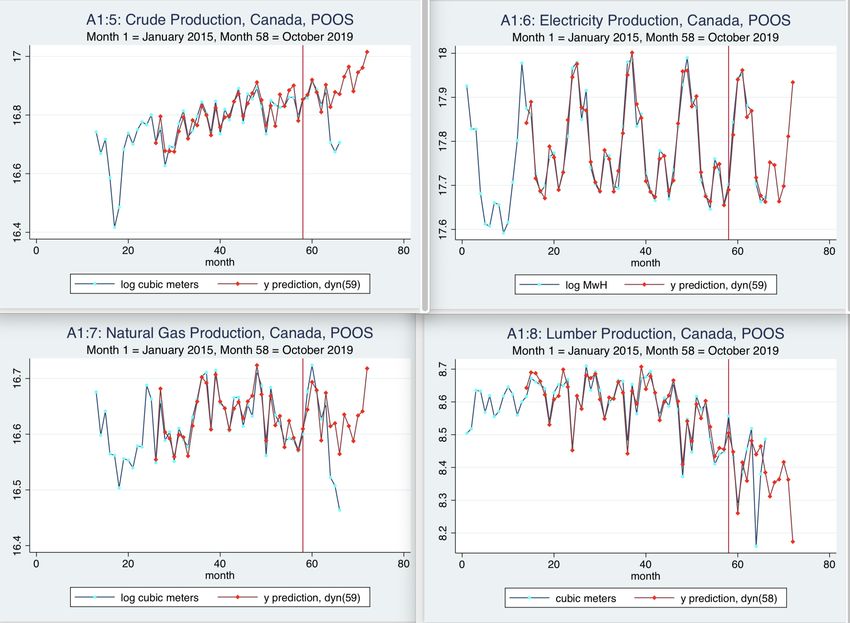
4   Margaret E. Slade

et al. (1996) to forecast expected deaths.4 That model fits seasonal effects and
trends to time–series data. The model itself — its functional form — is the
same for all infectious diseases, regions, and/or demographic groups. However,
the parameters of the model are fitted to the sample (disease, region, group)
of interest.
   In discussing its treatment of excess deaths, Statistics Canada (2020) notes
that not all excess deaths are directly due to COVID–19, since there are
indirect consequences, such as missed or delayed interventions and fewer
traffic accidents, that cause increases or decreases in mortality. Nevertheless,
a measure of the toll of the pandemic should account for both the direct and
indirect consequences. Of course, there are other causes of mortality. However,
those causes are assumed to follow normal patterns. All–cause mortality is
widely used by demographers and other researchers to understand the full
impact of deadly events, including epidemics, wars, and natural disasters.
   The loss measure of this paper shares many of the characteristics of the
excess–death measure. For example, I use the same model — the same
functional form — for each industry and province. However, its parameters
are fitted to each province/industry pair. Furthermore, output losses could be
directly affected by the virus due to for example, virus–related absences from
work, but there are also indirect consequences due to, for example, provincial
lockdowns. Predicted losses capture, and should capture, both sorts of effects.
Finally, there are unobserved causes of both mortality and output losses that
are unrelated to the virus and those factors are treated as noise.

3. The Industries and the Data
The data, which are from Statistics Canada, consist of all three–digit (or
equivalent) industries for which monthly data by province are collected. The
industries can be grouped into seven categories: nondurable manufacturing,
durable manufacturing, wholesale trade, retail trade, primary extraction and
harvesting, hospitality and tourism, and housing. However, the bulk of the
industries are in the first three categories. Specifically, there are eleven
nondurable and nine durable manufacturing industries, six wholesale, ten
retail, four primary, three hospitality and tourism, and one housing industry
series. The data appendix (A1) contains a more complete description of the
industries and the data.
   Industry rather than establishment data were chosen because that data are
publicly available and do not require the use of Statistics Canada Research
Data Centers, which were closed during the lockdown. Furthermore, unlike
results that use establishment data, results that are obtained from industry

4 Faust et al. (2020) is an exception. Those authors use a seasonal ARIMA model to
  forecast expected deaths in all US Health and Human Services regions by demographic
  group using data from 2015 to 2019.

Canadian Journal of Economics / Revue canadienne d’économique 20XX 00(0)
Many Losers and a Few Winners              5

data do not have to be vetted by Statistics Canada, which can be a lengthy
process.
    I use monthly time–series observations from January 2015 to February
2020 to estimate a forecasting model for each industry in each province. The
first period, which is somewhat arbitrary, was chosen to balance the tension
between having more observations and having more relevant observations.
Since data for the the first year are used to start the models, at least five
years are needed to estimate reasonable models.5
    Most of the observations are revenues (i.e., data for manufacturing,
wholesale, retail, and hospitality). Those data are deflated by the relevant
provincial consumer price index, all items. In contrast, data on the primary
industries, travel, and housing are in physical units. Nevertheless, since
percentage differences are compared, uniformity of units is not required.6
    When there are too few establishments in an industry, Statistics Canada
withholds observations. This practice, which was adopted for confidentiality
reasons, means that the data are incomplete and some industries cannot
be analyzed for some provinces.7 With respect to provinces, the Atlantic
Provinces, especially Newfoundland and Labrador and Prince Edward Island,
are the least complete. With respect to industries, manufacturing which is
the most concentrated, is the least complete. As a result, rather than having
390 (39 industries ◊ 10 provinces) time series, I have 292. In terms of output,
however, the coverage is much higher.

4. The Forecasting Mode and Preliminary Analysis
4.1. The Model
Rather than fitting a different time–series model for each industry and
province, which would involve making subjective judgment calls in each case, I
use a common parsimonious model that captures trend, seasonal, and cyclical
components. Suppose that Yijt is an outcome — an observation on production
in monetary or physical units — for industry i in province j and month t, y
is the natural logarithm of Y , and yijt is the first difference, yijt ≠ yijt≠1 . I
model the time–series behavior of y as
             1             12
     yijt = —ij L1 yijt + —ij L12 yijt + µm
                                          ij + “ij t + uijt ,                            (1)
where Ln denotes the nth lag of the variable that follows it, and for each ij, — 1
measures the sensitivity of the dependent variable to its value in the previous

5 Faust et al. (2020) use the same time period to estimate their forecasting model.
6 An exception is when there are systematic price movements — increases or declines —
  a possibility that is assessed in section 6.
7 When only one or two observations are missing, I estimate the missing points using the
  Kalman filter. In other words, if xt is missing, it is estimated as the expectation of that
  variable, given the history up to t ≠ 1. All time series in my data span the entire period.

           Canadian Journal of Economics / Revue canadienne d’économique 20XX 00(0)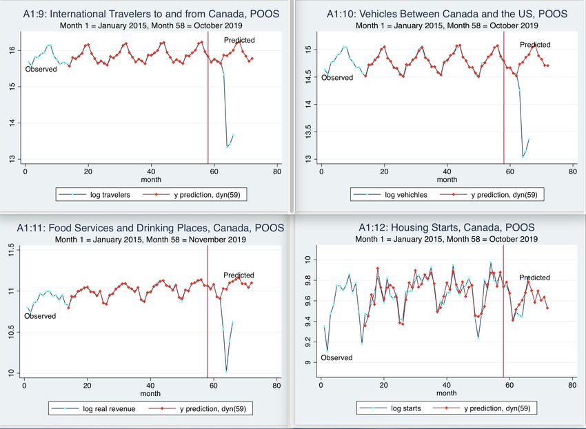
6   Margaret E. Slade

month, — 12 measures sensitivity of the dependent variable to its value in the
same month of the previous year, µm is a vector of monthly fixed effects, and
“ is the slope of the trend. This model is estimated for each industry and
province using data for January 2015 to February 2020.
   The functional form was chosen for both economic and econometric reasons.
The dependent variable, percentage changes in output or revenue, was chosen
to be independent of scale and comparable across sectors and regions. It also
has the advantage of stabilizing the variance by taking logs and removing
a unit root by differencing. The one and 12 month lags were chosen to be
consistent with common naive but sensible practices.
   To anticipate results, the coefficient of the one–period lag is often negative.
In particular, when activity is unusually high (a large positive percentage
change) or low (a large negative change) in one period, it tends to revert back
to normal (a percentage change of the opposite sign) in the next. In contrast,
the coefficient of the 12–month lag, which tends to be positive, allows for
longer term cycles. In other words, unusually high (low) activity can persist
for several years. In both cases, the effects decay with time: the absolute values
of the coefficients are less than one. Finally the seasonal fixed effects account
for normal monthly differences that are due, for example, to the fact that sales
are apt to incresase in December.
   It is also possible that there is a trend (higher or lower percentage changes
in each period) if, for example the industry is growling rapidly. However, the
coefficient of the trend tends to be insignificant.8 Of course, there is a great
deal of variation across industries and regions.
   For each i, j, and t, percentage prediction errors or losses (PL) are then
calculated for each time–series observation using the formula
                 Ŷijt ≠ Yijt
    P Lijt =                       ,                                                      (2)
               .5(Ŷijt + Yijt )
where ŷijt is the prediction of yijt from (1) and Ŷijt = eŷijt .9

8 The trend was kept because it is important in a few industries.
9 This is what Granger and Newbold (1976) call the naive forecast, not their optimal
  forecast. However, Luetkepohl and Xu (2012) conclude that optimal forecasts do not
  necessarily outperform naive forecasts because the former involve the forecast error
  variance, which is unknown and has to be replaced by an estimator. With respect to
  their simulations, they state that “Using the usual estimator for this quantity, the
  optimal predictor does not have an advantage over the naive predictor in samples of
  common size” p.637. Moreover, in table 2, which is the only table that compares the
  ratio of optimal to naive forecasts for different specifications of the simulations, in only
  one out of 40 cases does the optimal outperform the naive forecast. In addition, using
  real data, they find that naive forecasts outperform linear forecasts — the problem does
  not arise when variables are not logged — except in cases where taking logs destabilizes
  the variance. Furthermore, the gains that are associated with the naive forecasts can be
  dramatic.

Canadian Journal of Economics / Revue canadienne d’économique 20XX 00(0)
Many Losers and a Few Winners 7
The predictions of the dependent variable for the estimation period are
static in the sense that they use realized values of explanatory variables. In
contrast, for the forecast period — March to December of 2020 — dynamic
recursive forecasts are used to predict percentage changes using the Kalman
filter. In other words, instead of using realized values of lagged y to obtain ŷ
in (2), the expectation of yt conditional on the history up to tú is calculated,
where tú is February 2020 (tú = 62) and t > tú .
Like excess death calculations, this exercise is descriptive. The forecasts are
business as usual estimates that can be compared to what actually happened.
4.2. Preliminary Analysis
The estimated predicted losses are used in further analyses. Prior to that
assessment, however, one can get a feeling for the findings by examining
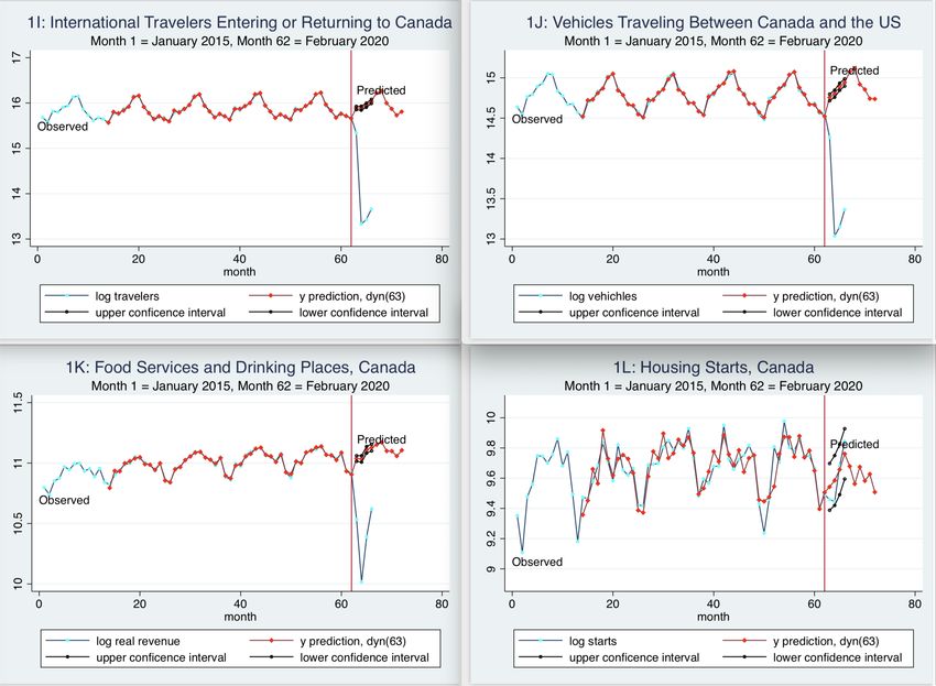
a set of graphs for Canada as a whole.10 Figure 1 contains graphs of the
nondurable manufacturing, durable manufacturing, wholesale trade, and retail
trade sectors as well as crude oil, electricity, natural gas, lumber, international
travel, vehicle border crossings, food services and drinking places, and housing
starts.11
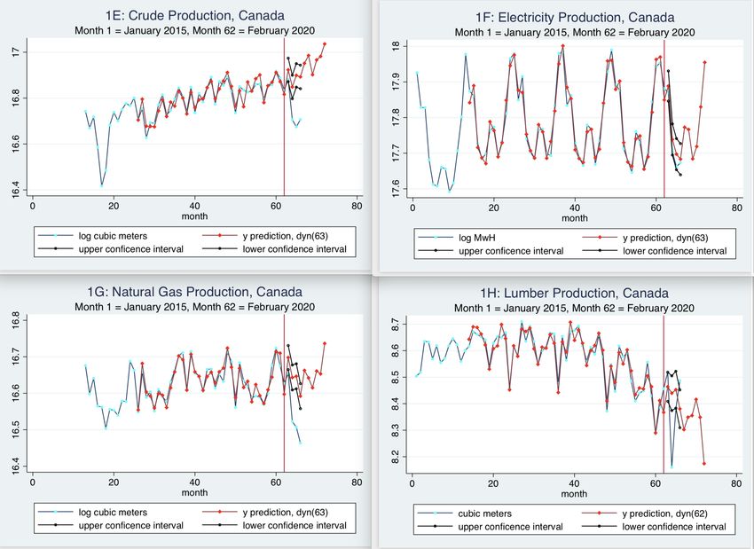
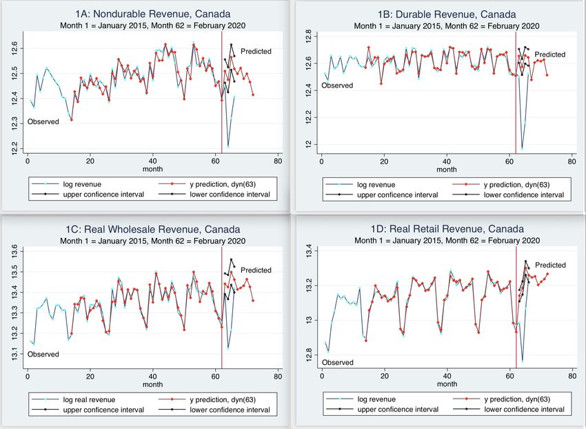
In each graph, points on the blue line are observed values, whereas points
on the red line are predictions from the model. The red line begins a year
after the blue because the first 12 months are used to start the model. The
vertical line indicates February 2020, the last month in the data that were
used to estimate the model. Forecasts up to this line are static, whereas after
the vertical line they are dynamic. The black lines are confidence intervals for
the dynamic (post–lockdown) forecasts.
A percentage loss in any post–lockdown month is approximately the
difference between the red and blue points for that month, whereas the total
loss is approximately the area between the red and blue lines. Predictably, the
graphs show that the hospitality and tourism sector (graphs 1:I–K) was the
hardest hit. Nevertheless, with the exception of housing starts and electricity,
all graphs show regions of the observed values that are significantly below the
forecasts.
Although it appears as though most industries began to recover in May,
that is not obvious since economic activity was often predicted to be higher
in May. For example, the uptakes in predicted and actual outputs in May
are approximately equal for nondurables and wholesale trade (1:A and 1:C),
whereas the realized increase is greater than the forecast for retail (1:D). By
10 Countrywide losses are not used in the later analysis where provincial losses are
assessed. Nevertheless, they convey a reasonable picture of the behavior of the
provincial time series.
11 Industries other than manufacturing, wholesale, and retail are not further aggregated
because the groups are measured either in physical units (e.g. energy and lumber) or
are in both physical and monetary units (e.g., international travel and food services
and drinking places).
Canadian Journal of Economics / Revue canadienne d’économique 20XX 00(0)8 Margaret E. Slade June, in contrast, most industries had recovered or had moved a long way in that direction. Nevertheless, food services and drinking places (1K) were only half way there, which reflects the restrictions that were placed on reopening those establishments. Finally, the recovery of international travel (1:I and J) was de minimis. The graphs in the figure 1 show that, in sample, the predictions from the model are fairly close to the observed data. However, those forecasts are one step ahead. Appendix A2 shows similar regressions where the last four in– sample data points — November 2019 to February 2020 – were not used in the estimation so that dynamic forecasts could start earlier. The figures show that, in contrast to the out of sample (OOS) forecasts for the pandemic period, the pseudo out of sample (POOS) or pre–pandemic forecasts fit the data well. The highly seasonal nature of the data illustrates why the previous month’s value is usually a poor comparison. The same month in the previous year is often a better predictor. However, when there are trends, that method also performs poorly. For example, graphs 1:E and 1:H show that crude oil production was expected to rise whereas lumber production was predicted to fall, relative to the previous year. 5. Analysis of Predicted Losses The first analysis of predicted losses by province and industry during the COVID–19 period involves a regression of those losses on industry–group and provincial fixed effects.12 The industry groups or sectors are: nondurables, durables, wholesale, retail, primary, tourism and hospitality, and housing. This analysis uses all 292 short and medium–run losses. Table 1 shows the results. The base case is Manitoba, the province that was least affected by COVID–19 in terms of short–run predicted losses, which implies that, for any province, the estimated provincial effect is net of the Manitoba effect. The regression does not contain a constant. The table has nine columns: the first indicates the province or industry group; the next three pertain to the short–term (losses in March), whereas the following three pertain to the medium–term (four–month–average losses). The three entries for each subperiod are the value (the estimated fixed effect), the standard error of that estimate, and the estimate’s rank. Finally, the last two columns show COVID–19 cases per capita and provincial ranks in terms of cases per capita, from highest to lowest.13 12 The dependent variable, predicted loss, was estimated in a prior stage and thus subject to measurement error. However, as it is the dependent variable, measurement error is included in the error term, causing the standard errors to be larger and my findings are thus conservative. 13 Provincial cases per capita are total cases up to July divided by provincial population. The data were obtained from the New York Times COVID–19 database. Canadian Journal of Economics / Revue canadienne d’économique 20XX 00(0)
Many Losers and a Few Winners          9

TABLE 1
Average Losses by Industry and Province

 P rovince     Loss               Loss   Av Loss              Av Loss    Cases per   Cases
               March              Rank   4–month              Rank       100,000     Rank
               (%)                       (%)

 QC            12.9úúú   (2.6)    1      13.6úú      (2.3)    2          696         1
 ON            10.0úú    (2.0)    2      12.4úú      (2.1)    3          276         2
 NS            9.5ú      (1.6)    3      10.4        (1.5)    4          116         4
 NL            9.3       (1.5)    4      9.8         (1.3)    5          50          7
 PE            9.2       (1.3)    5      14.0ú       (1.7)    1          25          9
 BC            7.6       (1.5)    6      4.4         (0.7)    8          68          6
 AB            6.5       (1.3)    7      8.7         (1.5)    6          221         3
 NB            4.9       (0.8)    8      4.8         ( 0.7)   7          22          10
 SK            2.5       (0.5)    9      -0.1        (-0.2)   10         80          5
 MB            0.0                10     0.0                  9          26          8

 Sector        Loss               Loss   Av Loss              Av Loss
               March              Rank   4–month              Rank
               (%)                       (%)

 TH            31.6úúú   (6.0)    1      88.6úúú     (13.9)   1
 RE            10.9úúú   (2.7)    2      16.6úúú     (3.4)    3
 HS            10.8      (1.4)    3      24.9úúú     (2.8)    2
 DU            -2.8      (-0.6)   4      8.8ú        (1.7)    4
 WH            -3.2      (-0.7)   5      4.8         (0.9)    6
 PR            -7.8      (-1.3)   6      -3.4        (-0.5)   7
 ND            -8.2      (-1.5)   7      5.4         (0.8)    5

               R2 0.41                   R2 : 0.66            Obs: 292

  Manitoba is the base province
  Cases per capita were measured in July
  t statistics in parentheses
  TH is tourism and hospitality, RE is retail, HS is housing starts, DU is durables, WH is
  wholesale, PR is primary, ND is nondurables
  ***, **, and * denote significance at 1%, 5%, and 10%, respectively

   Quebec and Ontario — which are the most populous provinces and had
the largest number of infections per capita — were the hardest hit in the
short term. With the exception of New Brunswick, the Atlantic provinces had
the second highest short–run losses, in spite of the fact that Newfoundland

             Canadian Journal of Economics / Revue canadienne d’économique 20XX 00(0)
10 Margaret E. Slade and Labrador and Prince Edward Island (PEI) had very few COVID–19 cases. The Western provinces of British Columbia (BC) and Alberta was the third group, and the Prairie provinces of Saskatchewan and Manitoba were the least affected. Nevertheless, only the first three short–run provincial– loss coefficients are statistically significant at 10% or higher. However, this simply means that the provincially–constant unobservable effects were not significantly different from the Manitoba–constant unobservable effect. Comparing the short and medium term, since the lockdown occurred in the middle of March, it is not surprising that most provincial losses are greater in the medium run. As the earlier figures show, however, the transitions were not smooth passages from bad to worse; instead, the dynamic pattern for most industries was U shaped. In addition, PEI moved up four ranks into the highest position whereas BC moved down two, which means that the recovery in PEI was slower, and that in BC faster, than average. In general, the consequences for the eastern provinces were more severe than for the western. Turning to the industry groups or sectors in Table 1, tourism and hospitality was by far the most affected, followed by retail and housing. However, only the first two short–run coefficients are significant. Housing starts are the most variable and difficult to predict, which accounts for the lack of significance of its short–run loss coefficient. Nevertheless, the housing loss became significant in the medium term. The remaining groups actually gained in the short run; the coefficients are negative. However, those gains were not significant and they mostly disappeared in the medium term. Finally, there were no large changes in industry ranks between the short and medium run. One reason why losses in manufacturing and wholesale were small and insignificant on average is that there is substantial variation within the sectors, with both losing and winning industries. In order to explore that heterogeneity, I assess the industries within three sectors: manufacturing, wholesale, and retail. Losses within the primary industries were also heterogeneous, with crude oil and natural gas suffering substantial losses while electricity and lumber fared better. However, there are insufficient observations within that group to perform a formal analysis. Finally, there is much more uniformity of losses within the remaining sectors. Three–digit industries in the manufacturing sector are more disaggregate than in the other two. For example, although food and beverages are combined into single three–digit wholesale and retail industries, they are separate three– digit manufacturing industries. For that reason I created subgroups within manufacturing.14 14 The subgroups in manufacturing are food and beverages; paper; printing; petroleum, chemicals, and plastics; wood products; nonmetalic, primary, and fabricated minerals; machinery; computers, electronics, and electrical; transportation equipment; and furniture. Canadian Journal of Economics / Revue canadienne d’économique 20XX 00(0)
Many Losers and a Few Winners           11

   Table 2 contains the results of three within–sector regressions of percentage
losses during the forecast period on industrial and provincial fixed effects for
both the short and medium run.15 Each part of the table shows a regression
that uses a different sample — manufacturing, wholesale, or retail — and
includes fixed effects for the industries that are in the relevant sector.
   First, consider manufacturing. Table 2:A shows that short–run production
of furniture, transportation equipment, and printing was significantly down.
In the medium run, those three plus three additional industries had
significant losses: petroleum, chemicals, and plastics; nonmetalic, primary, and
fabricated minerals; and computer, electronics, and electrical.16 In contrast,
manufacturing of food and beverages was significantly up in the short run.
However, that gain disappeared later on. Finally, although not statistically
significant, paper manufacturing was up in the short run. Presumably, the
latter was due to increased demand for household paper.
   Next, consider wholesale. Table 2:B shows that distribution of farm
products, motor vehicles and parts, and building materials was significantly
down in the short run. In the medium run, except for machinery and
equipment, all sectors suffered significant losses that range between 34% and
10%, and there were no gains.
   Finally, consider retail. Table 2:C shows that sales of clothing and
accessories; motor vehicles and parts; sporting goods, books, and music;
gasoline; furniture; and electronics and appliances were significantly down
in the short run and continued to be so after several months. Clearly the
retail sector was the hardest hit with significant medium term losses ranging
between 91% and 9%. Nevertheless, retail sales of food and beverages were
up significantly, with gains of 10.9% in the short and 7.5% in the medium
run. Increased retail sales occurred as consumers switched from dining out to
dining in.

15 Each of the three subgroups includes a miscellaneous category that is not used in the
   regressions.
16 The loss in the final group is driven by losses in the manufacture of appliances.

            Canadian Journal of Economics / Revue canadienne d’économique 20XX 00(0)
12 Margaret E. Slade
TABLE 2
Average Losses by Industry and Province, More Detailed Breakdown
Industry Loss Rank Av. Loss Rank
March 4–month
(%) (%)
A : M anuf acturing
FUR 19.5úúú (3.4) 1 32.3úúú (4.4) 3
TEQ 15.0úúú (2.6) 2 35.5úúú (4.8) 2
PRI 12.4ú (1.9) 3 36.6úúú (4.4) 1
PCP 4.9 (1.2) 4 21.8úúú (4.2) 4
NPFM 4.4 (1.4) 5 16.9úúú (4.1) 5
CEE 2.3 (0.5) 6 14.8úú (2.5) 6
ME -1.9 (-0.4) 7 7.2 (1.2) 7
WP -2.5 ( -0.6) 8 0.2 (0.3) 10
FB -8.0ú (-1.8) 9 1.6 (0.3) 8
PA -8.4 (-1.3) 10 0.6 (0.1) 9
Obs: 75 R2 : 0.32 R2 : 0.61
B : W holesale
FP 18.3úúú (4.9) 1 16.6úúú (3.3) 2
MVP 13.4úúú (4.6) 2 34.0úúú (7.9) 1
BM 6.6úú (2.2) 3 12.7úúú (3.0) 3
FB 2.4 (0.9) 4 9.8úú (2.4) 4
ME 0.9 (0.3) 5 3.3 (0.8) 6
HPC -2.2 (-0.6) 6 9.6ú (1.9) 5
Obs: 45 R2 : 0.57 R2 : 70
C : Retail
CLA 69.6úúú (25.8) 1 91.1úúú (27.3) 1
MVP 45.3úúú (16.8) 2 40.6úúú (12.2) 2
SBM 27.9úúú (9.8) 3 37.9úúú (10.8) 3
GA 21.7úúú (8.0) 4 31.7úúú (9.5) 5
FUR 20.7úúú (7.3) 5 36.1úúú (10.3) 4
EA 9.7úúú (3.6) 6 9.2úúú (2.8) 6
BMG 1.6 (0.6) 7 3.3 (0.9) 7
GM 1.3 (0.5) 8 0.0 (0.0) 9
HPC -3.6 (-1.4) 9 2.3 (0.7) 8
FB -10.9úúú (-4.0) 10 -7.5úú (-2.5) 10
Obs: 96 R2 : 0.93 R2 : 0.93
Canadian Journal of Economics / Revue canadienne d’économique 20XX 00(0)Many Losers and a Few Winners 13
Notes for table 2:
M anuf acturing :
FUR is furniture, TEQ is transport equipment, PRI is printing, PCP
is petroleum, chemicals, and plastics, NPFM is nonmetalic, primary, and
fabricated minerals, CEE is computers, electronics, and electricals, ME is
machinery and equipment, WP is wood products, FB is food and beverage,
PA is paper
W holesale :
FP is farm products, MVP is motor vehicles and parts, BM is building
materials, FB is food and beverage, ME is machinery and equipment, HPC is
household and personal care
Retail :
CLA is clothing and accessories, MVP is motor vehicles and parts, SBM
is sporting goods, books, and music, GA is gasoline, FUR is furniture, EA is
electronics and appliances, BMG is building materials and gardening, GM is
general merchandise (mostly department stores), HPC is health and personal
care, FB is food and beverage
t statistics in parentheses
***, **, and * denote significance at 1%, 5%, and 10%, respectively
Canadian Journal of Economics / Revue canadienne d’économique 20XX 00(0)14 Margaret E. Slade 6. Sensitivity Analysis Most of the findings that have been reported so far are consistent with prior expectations. However, the fact that the Atlantic provinces were hit so hard is a bit puzzling, given that cases per capita were low in three out of four of those provinces. One possible confounding factor is that data are missing for some industries in some provinces, and the problem is more acute for the Atlantic provinces, especially Newfound and Labrador and PEI. For that reason, I assess more aggregate industry data that are available for every province. For this analysis, aggregate revenues of nondurables, durables, wholesale, and retail, all of which are simple to aggregate, are included.17 In contrast, the quantity variables are less susceptible to aggregation.18 I therefore chose one time series from each group. Moreover, the chosen series — electricity, international travelers, and housing starts — are the only series in their respective groups that are complete for all ten provinces.19 Table 3, which contains the results of the more aggregate regressions, shows that, instead of reversing the results for the Atlantic Provinces, it confirms them. In particular, Newfoundland and Labrador is the hardest hit in both the short and medium run, with predicted losses of 34% and 49%, respectively. Moreover, comparing short and medium runs, PEI moves from rank 6 to rank 2 and BC falls from 5 to 7.20 As with the disaggregate data in Table 1, the sample splits between eastern and western provinces, with the former suffering more acutely. The sectoral results in Table 3 show that tourism, housing, and retail suffer the most in the short run and have significant losses in both periods. In particular, the number of international travelers, which is the most affected in both periods, suffered losses of 94% in the medium run. On the other hand, retail sales move from rank 3 to rank 5, reflecting their almost complete recovery by June. Finally, manufacturing, both durable and nondurable, show significant medium run losses that range between 22 and 19%. The fact that most of the data series are measured in value (P◊Q) whereas some — the primary industries, travel, and housing —are in physical units (Q) is another factor that could potentially bias the results. In particular, 17 The aggregation is performed by Statistics Canada and therefore includes the data that have been withheld. 18 One can aggregate the energy variables on a Btu basis. However, Statistics Canada does not do this and some of the data that would be required for the calculation are unavailable. 19 Some provinces do not produce all energy sources and/or lumber. In addition, Nova Scotia, PEI, and Newfoundland and Labrador do not have borders with the US and are the place of entry for almost no vehicles. 20 Provincial losses in Table 3 are higher than in Table 1 because Manitoba’s losses are not normalized to zero. Canadian Journal of Economics / Revue canadienne d’économique 20XX 00(0)
Many Losers and a Few Winners              15

TABLE 3
Average Losses by Industry and Province, Less Detailed Breakdown

 P rovince     Loss               Loss   Av Loss               Av Loss    Cases per    Cases
               March              Rank   4–month               Rank       100,000      Rank
               (%)                       (%)

 NL            34.0úúú   (3.4)    1      48.7úúú     (3.0)     1          50           7
 QC            23.4úú    (2.4)    2      45.5úúú     (2.8)     3          696          1
 NS            20.8úú    ( 2.1)   3      40.9úú      (2.5)     4          116          4
 ON            19.2ú     (1.9)    4      38.1úú      (2.4)     5          276          2
 BC            17.7ú     (1.8)    5      31.8úú      (2.0)     7          68           6
 PE            16.9ú     (1.7)    6      46.1úúú     (2.9)     2          25           9
 SK            10.6      (1.1)    7      21.5        (1.3)     10         80           5
 AB            9.2       (0.9)    8      33.3úú      (2.1)     6          221          3
 MB            7.7       (0.8)    9      23.1        (1.4)     9          26           8
 NB            4.6       (0.5)    10     31.4ú       (1.9)     8          22           10

               R2 0.33                   R2 : 0.43             Obs: 80

 Sector        Loss               Loss   Av Loss               Av Loss
               March              Rank   4–month               Rank
               (%)                       (%)

 TR            40.4úúú   (7.5)    1      93.7úúú     (14.9)    1
 HS            18.0úú    (2.4)    2      32.6úúú     (3.7)     2
 RE            15.3úú    (2.0)    3      16.7ú       (1.9)     5
 DU            9.6       (1.3)    4      19.3úú      (2.2)     4
 ND            5.8       (0.8)    5      21.7úú      (2.4)     3
 WH            3.3       (0.4)    6      12.1        (1.4)     6
 EL            -1.7      (-0.2)   7      -1.5        (-0.2)    7

               R2 0.48                   R2 : 0.77             Obs: 80

  For each province, observations on nondurables, durables, retail, and wholesale in this table
  pertain to totals across industries in the sector
  Cases per capita were measured in July
  t statistics in parentheses
  TR is international travelers, HS is housing starts, RE is retail, DU is durables, ND is
  nondurables, WH is wholesale, EL is electricity,
  ***, **, and * denote significance at 1%, 5%, and 10%, respectively

             Canadian Journal of Economics / Revue canadienne d’économique 20XX 00(0)
16 Margaret E. Slade unmeasured price changes could be systematic and large. For example, the price of crude oil became very low during the period, which means that the quantity measure is an overestimate. To see if this makes a difference, a regression that is similar to that in table 1 but omits the primary and housing industries was run. The travel industries were included because visitors do not have a market price that could change. When the regression without primary and housing was run, the group of four provinces that were hardest hit in the four–month period — Quebec, Ontario, PIE, and Nova Scotia — did not change. In addition, the group of four that were least hard hit — New Brunswick, BC, Saskatchewan, and Manitoba — also remained the same. However, in the middle, Alberta changed places with Newfoundland and Labrador and joined the top five. This change is probably due to the fact that crude oil production is an underestimate of the true impact on the oil industry. Nevertheless, the crude–oil price change was caused by long–run factors that were, to a large extent, independent of the pandemic. However, the drop in gasoline sales downstream during the lockdown exacerbated those factors. Still, since the change occurs in the middle of the rankings, it does not invalidate my principal conclusions. The results of this regression are in appendix A3. 7. Economic Responses by the Provinces Tables 1 and 3 compare the economic consequences — industrial losses — to the severity of the virus — cases per capita. However, there is no robust reason for the two to be positively correlated. Indeed, if higher cases per capita early on led to stronger provincial responses in the form of lockdowns and economic restrictions, greater provincial losses would have resulted. In contrast, those responses might have led to fewer cases of the virus later on. Even though the reduction in work hours due to illness would have had some effect on industrial output, it is likely that the effect of the economic restrictions dominated, or at least complemented, the employment effect. As with the excess deaths literature, my research seeks to evaluate both the direct — output loss due to illness — and indirect — output loss due to provincial responses — effects. In this section, I examine the indirect effects more closely. Most of the virus–related aid to workers and businesses in Canada came from the federal government and federal policy was uniform across provinces. Although the provinces did provide some relief, much of that relief was an attempt to bridge the gap until federal aid arrived or to reach households and individuals that were not eligible for federal support. In contrast, with the exception of closing the border to many forms of international travel, lockdowns and other restrictions were imposed by the provinces, who also bore the consequences. Canadian Journal of Economics / Revue canadienne d’économique 20XX 00(0)
Many Losers and a Few Winners               17

TABLE 4
Provincial COVID–19 Responses

  P rovince     March date         Number of cases     Number of restrictive    March date of
                when emergency     when emergency      measures adopted         first restriction
                declared           declared

  NL            19                 < 25 +              11 +                     11 +
  PE            16   +             < 25 +              12 +                     14
  NS            22   -             < 25 +              10                       8+
  NB            19                 < 25 +              12 +                     10 +
  QC            14   +             < 25 +              12 +                     11 +
  ON            17                 189 -               12 +                     8+
  MB            20   -             < 25 +              11 +                     15 -
  SK            18                 < 25 +              9-                       11 +
  AB            17                 97                  10                       15 -
  BC            17                 186 -               6-                       16 -

                                                       Source: Breton and Tabbara (2020)
    + indicates more restrictive, - indicates less restrictive
    Date emergency declared: March 14–16 is early, March 20–22 is late
    Number of cases: Low is < 25, High is > 180
    Number of restrictions is out of 15
    Number of retrictive measures: 11–12 is high, 6–9 is low
    Date of first restriction: March 8–11 is early, March 15–16 is late

   Table 4 summarizes an attempt to measure the severity of the provincial
restrictions.21 Since reductions in output are the focus of this article, I have
chosen to limit my analysis to policies that restrict economic activity.22 A +
in the table means that the related variable was relatively more restrictive
whereas a - means that it was less. All dates are in March.
   The first and most important response was a declaration of a state of
emergency or public health emergency.23 All ten provinces declared states

21 The data in table 4, which comes from Breton and Tabbara (2020), was supplied by
   Charles Breton.
22 For this reason, I do not include, for example, restrictions on visits to long–term care
   homes, which were also imposed by the provinces.
23 Although a state of emergency differs from a public health emergency — the first gives
   broad powers to the premier or governor in council whereas the second gives them to
   the health minister or public health officer — I make no distinction between the two
   here.

              Canadian Journal of Economics / Revue canadienne d’économique 20XX 00(0)
18 Margaret E. Slade of emergency within a 9–day period. Nevertheless, nine days can make a substantial difference, particularly in the first few weeks. The first column in table 4 shows the province, the second indicates the date on which an emergency was declared, and the third shows the number of virus cases per capita on that day. A plus in column two means an emergency was declared on an early date (March 14–16) whereas a minus indicates a late date (March 20–22). In column three, a plus means that cases were low when emergency was declared (less than 25 or an early response) whereas a minus means that they were high (over 180 or a late response). The third and fourth columns in table 4 contain information about the number of restrictions imposed by each province and the date of the first imposition. Restrictions can be, for example, various sorts of closures, travel restrictions, or fines for violations of those restrictions. Table 5 lists the complete set of fifteen restrictions. In column four of table 4, eleven or more restrictions is considered high (+), whereas nine or less in considered low (-). Finally, March 11 or before is considered an early imposition (+) whereas March 15 or later is considered late (-) If one sums the pluses net of the minuses across columns in the table, it shows that Quebec, which was hardest hit economically also had the most restrictive policy (four pluses and no minuses), followed by PEI, Newfoundland and Labrador, and New Brunswick (3 pluses and no minuses). In contrast, the three western provinces of Manitoba, Alberta, and BC were the least restrictive (net 0, -1, and -3, respectively). This analysis is clearly highly descriptive and lacking in rigor. Nevertheless, it sheds light on why the Atlantic Provinces were hit hard relative to the western provinces. Finally, differences in the effects of the restrictions across industries are more obvious. For example, the restrictions on international travel, which were severe, led to the almost complete shut down of that sector. Furthermore, nonessential retail closures led to the initial severe decline in retail sales, whereas reopening with restrictions resulted in the partial recovery of that sector. One should not interpret these findings as evidence that lockdowns and other restrictions are bad. Clearly they are bad for business. However, there is a short–term tradeoff between economic and health outcomes. Moreover, one can hope that short term losses lead to long term gains in the form of faster recovery as the virus disappears more quickly. 8. Final Remarks All of the provinces suffered severe losses due to COVID–19. However, the burden was uneven. Losses in Quebec and Ontario — the provinces with the largest populations and highest number of cases per capita — were in the group that was most heavily impacted. Less expected, however, the Atlantic provinces of Nova Scotia, PEI, and Newfoundland and Labrador, which rank Canadian Journal of Economics / Revue canadienne d’économique 20XX 00(0)
Many Losers and a Few Winners   19

TABLE 5
Restrictive Measures

 Closed primary and secondary schools
 Closed nonessential business
 Closed restaurants except take out
 Restricted restaurant capacity
 Closed bars
 Closed gyms
 Closed daycares
 Closed movie theaters
 Closed cannabis and liquor stores
 Ordered self isolation for domestic travelers
 Interprovincial checkpoints
 Intra–provincial travel restrictions
 Fines for not respecting social distancing
 Fines for not respecting self isolation
 Fines for profiteering

                                             Source: Breton and Tabbara (2020)

low in population and cases per capita, were also in that group. This finding
can be partially explained by the fact that those three provinces depend
heavily on tourism. That is not the whole story, however, as they also suffered
large losses in other sectors. Furthermore, the recovery in PEI was slower than
in the other provinces in the top group.
   Digging deeper, I examine and quantify the effects of provincial economic
responses to the virus, such as lockdowns, travel restrictions, and fines. Those
policies are perhaps more highly correlated with output losses than are cases
per capita. Indeed, it is likely that the imposition of lockdowns and other
economic restrictions had a bigger impact on industrial activity compared to
the direct reductions due to illness.
   Data on the number and types of restrictions as well as the dates when
those restrictions were imposed is used to classify the severity of provincial
economic responses. That descriptive analysis sheds light on why the Atlantic
Provinces, which adopted more restrictive policies earlier on, suffered large
losses compared to the western provinces.
   Along with housing starts, the service sectors of tourism, hospitality,
and retail, which are the sectors with highest person–to–person contact,
suffered the most. Nevertheless, within retail, sales of food and beverages
were significantly up. Furthermore, within–sector disparities were large. For
example, whereas restaurants and bars lost over 90% of their revenues in

          Canadian Journal of Economics / Revue canadienne d’économique 20XX 00(0)
20 Margaret E. Slade April and around 50% on average, retail sales of food and beverages were up by approximately 11% in March and 8% on average, reflecting a shift from restaurant to home dining. The non–service sectors of manufacturing and wholesale suffered less on average. However, as with retail, there were large within sector differences. On average, the primary industries were least affected. However, at the maximum, crude oil production was down by 22%. In contrast, maximum gasoline sales losses were more than 60%. This discrepancy can be explained by the fact that, unlike gasoline sales that are easy to adjust, it is very costly to close a refinery and there was a glut of crude oil on the market that resulted in low prices. The energy industries were therefore not winners. In Canada, as in the US, public policies in response to the virus, such as the timing and duration of lockdowns, the list of essential industries that are not subject to lockdown, the wearing of face masks, and limitations on the size and locations of gatherings, are governed by the provinces. Since the provinces bear the costs and consequences of most of those activities, rather that adopting blanket policies, the federal government should aim to alleviate conditions in the regions that were most adversely impacted. To the extent that federal policy has targeted the firms and households that are most negatively impacted rather than handing out uniform subsidies, that has been the case.24 In contrast to restrictive responses that mostly reduce output, most virus– related subsidies to industries and sectors of the economy were federally mandated. As we have seen, the impact of the virus on types of businesses was far from equal. To illustrate, restaurants and bars were heavily impacted and most of those establishments are small. Furthermore, since large department stores and retail chains were better equipped to sell online,25 the problems facing small retailers were more severe.26 Those facts point to the desirability of increasing subsidies to small businesses, particularly those that are very small. Unfortunately, it may be too late to rescue many of the establishments that were hit the hardest. 24 In contrast, the US relied much more heavily on uniform subsidies to households. 25 For example, after retail food and beverages, general merchandise, which is mainly department stores, was the least affected industry. Nevertheless, during the first wave, large retail chains, such as Aldo, Pier 1, and Reitmans, filed for bankruptcy, closed many stores, or laid off most of their employees. More recently, even The Bay has closed some of its retail stores. 26 For more evidence on the differential impact of the virus on small businesses, see Fairlie (2020). Canadian Journal of Economics / Revue canadienne d’économique 20XX 00(0)
Many Losers and a Few Winners         21

References
Abay, K. A., K. Tafere, and A. Woldermichael (2020) “Winners and losers
  from COVID–19: Global evidence from Google search,” World Bank Policy
  Research Working Paper 9268
Aguirregabiria, V., J. Ga, Y. Luo, and P. Mira (2020) “A dynamic structural
  model of virus diffusion and network production: A first report,” C.E.P.R.
  Discussion Paper DP14750
Bartik, A., M. Bertrand, Z. Cullen, E. Glaeser, M. Luca, and C. Stanton
  (2020) “How are small businesses adjusting to COVID–19? Early evidence
  from a survey,” NBER Working Paper W26989
Breton, C., and M.-D. Tabbara (2020) “How the provinces compare in their
  COVID–19 responses,” Policy Options article
Brodeur, A., A. Clark, S. Fleche, and N. Powdthavee (2020) “COVID–19,
  lockdowns, and well being: Evidence from Google Trends,” University of
  Montreal Economics Working Paper 2004E
Casares, M., and H. Khan (2020) “A dynamic model of COVID–19: Contagion
  and implications of isolation enforcement,” Carleton Economics Working
  Paper 20–02
Fairlie, R. (2020) “The impact of COVID–19 on small business owners:
  Evidence from the first three months after widespread social–distancing
  restrictions,” Journal of Economics and Management Strategy 29, 727–740
Farrington, C., N. Andrews, A. Beale, and M. Catchpole (1996) “A statistical
  algorithm for the early detection of outbreaks of infectious disease,” Journal
  of the Royal Statistical Society. Series A 159(3), 547–563
Faust, J., H. Krumholz, C. Du, K. Mayles, Z. Lin, C. Gilman, and R. Walensky
  (2020) “All cause excess mortality and COVID–19 related mortality among
  adults aged 25–44 years, March–July,” JAMA Research Letter
Ginsburgh, V., G. Magerman, and I. Natali (2020) “COVID–19 and the role of
  economic conditions in French regional departments,” ECARES. Working
  Paper 2020–17
Granger, C., and P. Newbold (1976) “Forecasting transformed series,” Journal
  of the Royal Statistical Society. Series B 38(2), 189–203
Jones, S. R., F. Lange, C. Riddell, and C. Warman (2020) “Waiting for
  recovery: The Canadian labor market in June 2020,” Canadian Public
  Policy
Lemieux, T., K. Milligan, T. Schirle, and M. Skuterud (2020) “Initial impacts
  of the COVID–19 pandemic on the Canadian labour market,” Canadian
  Public Policy
Luetkepohl, H., and F. Xu (2012) “The role of the log transformation in
  forecasting economic variables,” Empirical Economics 42(3), 619–638
Mohammed, A., R. M. Johnson, and C. van der Linden (2020) “Public
  responses to policy: The case of mask usage in Canada during COVID–
  19,” Canadian Public Policy

         Canadian Journal of Economics / Revue canadienne d’économique 20XX 00(0)
22 Margaret E. Slade Qian, Y., and S. Fulller (2020) “COVID–19 and the gender gap among parents of young children,” Canadian Public Policy Statistics Canada (2020) “Excess mortality in Canada during the COVID–19 pandemic,” Https://www150.statcan.gc.ca/n1/pub/45-28- 0001/2020001/article/00076-eng.htm Canadian Journal of Economics / Revue canadienne d’économique 20XX 00(0)
Many Losers and a Few Winners         23

Appendix A1: Data Appendix
All of the time–series data are from Statistics Canada and are publicly
available on their web page, https://www150.statcan.gc.ca/n1/en/type/data.
I chose all time–series that pertain to industrial activity, are available for
the country and the provinces, and are published monthly. Unfortunately,
some series are highly incomplete and are unusable (e.g., textile mills, textile
products, clothing manufacturing, leather manufacturing, and coal mining).
However, when data for two or more provinces were almost complete, that
industry was kept in the data. Moreover, when only one or two observations
were missing in a series, those observations were estimated using the Kalman
filter (see footnote 7). This means that all 292 series in the final data set are
complete. Finally, series that are labeled ‘miscellaneous’ are not used in the
analysis in section 5.
    Information on the complete set of industries that is included in the data
can be found in table A1.
    Most of the observations are revenues (i.e., data for manufacturing,
wholesale, retail, and hospitality). Those data are deflated by the relevant
provincial consumer price index, all items, also from Staitistics Canada. In
contrast, data on the primary industries, travel, and housing are in physical
units. Since percentage differences are compared, uniformity of units is not
essential. Nevertheless, I estimated a regression that eliminates most of the
physical unit data (see section 6 and appendix A3).
    The data on economic restrictions and the dates on which they were
adopted were supplied by Charles Breton.

Appendix A2: Pseudo Out of Sample Forecasts
The graphs in figure A1:1–12 are similar to those in figure 1:A–L except for
the fact that, with the former, the last four observations in the pre–pandemic
period were withheld from the estimation and the dynamic forecasts start in
November of 2019. The first four dynamic predictions are pseudo out of sample
(POOS) forecasts whereas the last four are out of sample (OOS) forecasts.

Appendix A3: Additional Sensitivity Analyses
Table A2 contains the results of a regression that omits the quantity variables
with the exception of travel (see the discussion in section 6). For ease of
comparison, the entries are in the same order as in table 1.

          Canadian Journal of Economics / Revue canadienne d’économique 20XX 00(0)
You can also read


