Measuring and Disentangling Ambiguity and Confidence in the Lab - MDPI
←
→
Page content transcription
If your browser does not render page correctly, please read the page content below
games
Article
Measuring and Disentangling Ambiguity
and Confidence in the Lab
Daniela Di Cagno 1 and Daniela Grieco 2, *
 1   Department of Economics and Finance, Luiss Guido Carli, 00198 Rome, Italy; ddicagno@luiss.it
 2   Department of Economics, Bocconi University, 20136 Milano, Italy
 *   Correspondence: daniela.grieco@unibocconi.it; Tel.: +39-338-462-8960

 Received: 7 December 2018; Accepted: 28 January 2019; Published: 18 February 2019

 Abstract: In this paper we present a novel experimental procedure aimed at better understanding the
 interaction between confidence and ambiguity attitudes in individual decision making. Different
 ambiguity settings not only can be determined by the lack of information in possible scenarios
 completely “external” to the decision-maker, but can also be a consequence of the decision maker’s
 ignorance about her own characteristics or performance and, thus, deals with confidence. We design
 a multistage experiment where subjects face different sources of ambiguity and where we are able to
 control for self-assessed levels of competence. By means of a Principal Component Analysis, we obtain
 a set of measures of “internal” and “external” ambiguity aversion. Our regressions show that the
 two measures are significantly correlated at the subject level, that the subjects’ “internal” ambiguity
 aversion increases in performance in the high-competence task and that “external” ambiguity aversion
 moderately increases in earnings. Self-selection does not play any role.

 Keywords: ambiguity; confidence; competence; precision; self-selection

 JEL Classification: D81; C91

1. Introduction
      Several real-life decisions have to be taken on the basis of probability judgments where the
information needed by the decision-maker is partially or totally missing. This lack of information
can derive from the ambiguity of the possible scenarios, odds, and payoffs, or it can result from
ignorance on the individual’s absolute performance or relative position as compared to other
individuals’ characteristics or performance. In the former situation, the type of ambiguity affecting the
decision-making process is generated by instances that are external to the individual. In the latter case,
ambiguity derives from the difficulty the individual experiences when evaluating her own capabilities
or traits or knowledge and is therefore strongly connected with her degree of (absolute or relative)
confidence. When it is the performance that matters, the decision to take part in a task can change
dramatically according to self-evaluation: people are rarely well-calibrated and often show “over-”
or “under-confidence”, and the presence of both biases is likely to modify the perceived degree of
ambiguity affecting their decisions. Moreover, when individuals have to self-evaluate with respect
to peers, this potential confidence bias is exacerbated by the additional difficulty of estimating peers’
performance or characteristics or knowledge and of individuating one’s own reference-group.
      This paper experimentally addresses the issue of ambiguity and confidence jointly within a unique
experimental framework. In particular, it aims at disentangling the effects of internally-generated
and externally-generated ambiguity situations on individual decision making by controlling for
self-assessed levels of competence.

Games 2019, 10, 9; doi:10.3390/g10010009                                       www.mdpi.com/journal/games
Games 2019, 10, 9 2 of 22
As for confidence, the experimental design allows the authors to measure the three types of
overconfidence introduced by Moore and Healy (2008)—overestimation, overplacement and overprecision [1].
As for ambiguity, the subjects’ ambiguity attitude is measured by using both a ‘willingness-to-bet’ paradigm
(choice between lotteries) and a ‘willingness-to-invest’ paradigm (investment choice) in order to control
for framing effects. For the first time to the best of our knowledge, a Principal Component Analysis
is performed to examine the behavioral consequences of internally-generated and externally-generated
ambiguity. A regression analysis shows that the measure of internal and external ambiguity aversion are
significantly correlated. However, while the latter positively depends on performance, the former positively
depends on earnings and negatively depends on the perceived ease of the experiment.
Very few studies address the issues of ambiguity and confidence jointly. Both phenomena are not
easy to measure, might present unclear responses to monetary incentives, interact with risk-attitude,
and could be strongly context-dependent. An exception is represented by Brenner et al. (2011)’s
paper on financial decisions in which the authors derive a model based on the max-min ambiguity
framework [2] that links overconfidence to ambiguity aversion and predicts that overconfidence is
decreasing in ambiguity (i.e., the more a portfolio’s returns are ambiguous, the less overconfident
investors are). Their experimental findings support this prediction. In a lab experiment with MBA
students, Shyti (2013) [3] investigated the choices of overconfident decision makers when dealing
with uncertain options whose outcomes have different likelihoods, finding that only overconfident
decision makers choose less uncertain options for low-likelihood outcomes, thus, not matching the
standard Prospect Theory predictions. The relationship between ambiguity and confidence has also
been studied in the context of gender differences. In a financial decision context, Gysler et al., (2002) [4]
found a significant and positive relationship between individual overconfidence and competence
measures that produces opposite effects according to the gender of the subject. In a framework aimed
at reproducing trading activities, Yang and Zhu (2016) [5] show that traders who think they are on
average better in terms of trading ability trade more when prior information about the distribution is
ambiguous, with a stronger effect for males.
Recent studies on confidence in one’s own knowledge (Blavatskyy, 2009) [6] have emphasized
the need to provide the subjects with proper financial incentives in order to elicit their actual beliefs
on one’s capabilities: despite the popularity of elicitation of confidence intervals, some authors (e.g.,
Cesarini et al., 2006) [7] have shown that this methodology might cause the deliberate misreporting of
confidence intervals due to strategic reasons. Furthermore, risk aversion (and in general risk attitudes)
might “dramatically affect the incentives to correctly report the true subjective probability of a binary
event, even under Subjective Expected Utility” ([8], p. 1).
A possible way to relate ambiguity and confidence is interpreting confidence as an “internal”
source of ambiguity (affecting an individual’s decisions), as opposed to “external” sources where the
lack of information is not about the decision-maker and her own characteristics. This is coherent with
Abdellaoui et al. (2011) [9] who define a source of uncertainty as concerning a group of events that is
generated by a common mechanism of uncertainty1 .
The way we relate ambiguity to confidence is also in line with Attanasi, et al. (2014)’s belief elicitation
under ambiguity [11], where ambiguity is generated in a two-stage setting à la Klibanoff, et al. (2005) [12]
by relying on different “external” sources in the first stage (i.e., binomial distribution, uniform distribution,
unknown distribution) at a between-subject level. Each external source is generated by a common
mechanism of uncertainty at a within-subject level. Then, given the second-stage urn composition (which
is unknown), the subjects’ beliefs about it are elicited. The heterogeneous distribution of beliefs they obtain
1 In Ellsberg’s (1961) [10] classical two-color paradox, the source of uncertainty can be represented by the color of a ball drawn
randomly from an urn containing 50 black and 50 red balls (the known urn), or by the color of a ball drawn randomly from
an urn with 100 black and red balls in unknown proportion (the unknown urn). Alternatively, other sources of uncertainty
could be Stock indexes like the Dow Jones index or the Nikkei index (with the foreign index implying a higher level of
uncertainty for a US resident due to the “home bias”).Games 2019, 10, 9 3 of 22
can be interpreted as an “internal” source of ambiguity, i.e., different levels of “confidence” for different
subjects. They find no correlation between this “confidence” and the subjects’ behavior under ambiguity.
Overconfidence is a well-established bias where subjective confidence in one’s judgment is
systematically stronger than objective accuracy. Despite the fact that most prior research has treated
different types of overconfidence as one and the same, this distortion takes different forms according
to the way accuracy in judgment is measured and categorized, as subjects are rarely overconfident in
every confidence category. A comprehensive classification has been introduced by Moore and Healy
(2008) [1], who suggest three categories: overestimation, which occurs when people think they are better
than they actually are; overplacement, which we observe when people think they are better than their
peers; overprecision, which happens when people think they are better in judging their performance
than they actually are or than their peers.
To the best of our knowledge, although there exist some experimental attempts to infer
individual confidence about one’s performance (as it will be reported below in detail) and to measure
overestimation, overplacement and overprecision, none of them has been implemented in order to
measure their effects on risk or ambiguity attitudes. On the contrary, two articles that have studied the
effects of overconfidence on risk attitudes. Both these studies focus on voting choice, modeling it as a
risky lottery. Attanasi at al. (2014) study subjects’ overconfidence and its relation with risk aversion in
a theory-driven experiment where each subject can get an informative signal about the others’ voting
preferences [13]. Attanasi et al. (2017) [14] explicitly refer to Moore and Healy (2008) [1], and show
how to incorporate overprecision into an expected utility framework and derive predictions about the
preferred majority threshold of a risk-averse and overconfident (over-precise) decision maker.
1.1. Overestimation
Overestimation typically emerges when subjects are badly-calibrated in assessing their own
absolute performance in a task or in a set of tasks. Literature in psychology provides evidence in favor
of systematic miscalibration and hard-easy effect (e.g., Lichtenstein and Fischhoff, 1977; Juslin et al.,
2000; Merkle, 2009) [15–17]. A typical non-incentivized assessment of beliefs asks subjects to predict
their performance or their probability of success. A common finding is that on questions perceived
as easy (where the success rate is high), the average confidence is substantially lower than the actual
success rate, whereas in questions perceived as hard (with a lower success rate), the average confidence
is substantially higher than the actual success rate: presenting subjects with easy vs. hard tasks is a
typical way to induce under- vs. overconfidence in the lab.
Recent incentivized measurements in economic experiments have revealed different patterns.
Blavatskyy (2009) [6] does not directly elicit estimation measures, but infers underconfidence in the
sense of underestimation from the choice of a payment scheme: either one question is selected at
random and the subject receives a payoff if she answers this question correctly, or the subject receives
the same payoff with a stated probability set by the experimenter to be equal to the percentage of
correctly answered questions (although the subject does not know this is how the probability is set).
The majority choose the second payment scheme, which she interprets as reflecting underestimation.
Urbig et al. (2009) [18] elicited confidence about one’s performance over a set of ten multiple
choice quiz questions using an incentivized mechanism that relies on probability equivalents for bets
based on one’s performance: their findings show almost no miscalibration since the average elicited
probability equivalent is extremely close to the actual rate of success.
Both Blavatskyy (2009) [6] and Urbig et al. (2009) [18] noted the difference between their findings
and those from the earlier psychology literature, and speculate that the difference may be due to the
introduction of incentivized elicitation devices.
Clark and Friesen (2009) [19] studied the subjects’ confidence via a set of tasks using either
non-incentivized self-reports or quadratic scoring rule (QSR) incentives, including two types of real
effort tasks involving verbal and numerical skills. They found underestimation more prevalent than
overestimation and better calibration with incentives, with underestimation being stronger amongGames 2019, 10, 9 4 of 22
those where higher effort is needed. One potential limitation of their analysis, however, is that unless
the subjects are risk neutral, QSR may result in biased measurements of confidence (we return to this
point below in more detail).
Murad et al. (2016) [20] used two elicitation procedures: self-reported (non-incentivized) confidence
and an incentivized procedure that elicits the certainty equivalent of a bet based on performance: the
former reproduces the “hard-easy effect”, whereas the latter produces general underconfidence, which is
significantly reduced, but not eliminated when the effects of risk attitudes are filtered out.
1.2. Overplacement
Overplacement deals with relative position and social comparison. In his seminal work, Festinger
(1954) [21] posited that people experience difficulty in testing their own ability against an objective
standard and therefore reduce this uncertainty by using the abilities of others as the subjective reality.
Overplacement has been observed in several domains where the “unrealistically high appraisals
of one’s own qualities versus those of others” emerges (Belsky and Gilovich, 1999 [22]); research
on overplacement has not only been categorized as research on ‘overconfidence’2 but also on the
‘better-than-average’ effect. Subjects who overplace themselves are asked to rate their characteristics
or performance in relative terms with respect to peers, and typically rate themselves as better than
average. The vast majority of studies measures overconfidence without providing subjects incentives
to assess their evaluation correctly (for a review of this literature, see Alicke and Govorun, 2005 [24]).
Research presenting the most impressive findings of overplacement has tended to focus on
simple domains, such as driving a car or getting along with others (College Board, 1976–1977 [25];
Svenson, 1981 [26]). Among the studies that measure overconfidence on how individuals’ beliefs on
their performance translate into the probability of winning, Camerer and Lovallo (1999) [27] infer
overplacement from subjects’ decision to enter a market of defined capacity when survivors have to
be relatively better than their peers in a task they self-selected into. Grieco and Hogarth (2009) [28]
investigate participants’ choice of betting on their own relative performance in a task or on a 50/50
risky lottery without knowing how well they did.
1.3. Overprecision
Overprecision can be defined as “the excessive faith that you know the truth” (Moore et al.,
2019 [29]) and leads us to rely on our own judgment too much, despite its many flaws (ibidem).
Among the practical economic consequences, the empirical evidence supports the failure to protect
from risks (Silver, 2012 [30]), the neglect of others’ perspectives and the failure to take advice (Minson
and Mueller, 2012 [31]), too high a willingness to trade (Daniel et al., 2001 [32]), and too little a search
for ideas, people and information (Haran et al., 2013 [33]). This is a robust3 and well-documented
phenomenon—although the less studied form of overconfidence—but lacks a full explanation and
is measured in such a way that can lead to biases. In a typical psychological study of calibration,
a participant answers a number of questions or makes a series of forecasts about future events and,
for each item, expresses a subjective probability that the chosen answer or forecast is correct. A person
is considered well-calibrated if there is a precise match between subjective assessments of likelihood
and the corresponding empirical relative frequencies.
Laboratory studies of overprecision typically use two paradigms for eliciting beliefs. The former
is the “Two Alternative Forced Choice Approach” (Griffin and Brenner, 2004 [34]): subjects choose
between two possible answers to a question and indicate the probability that the chosen answer is
correct. Empirical evidence (e.g., Kern, 1997 [35]) shows that subjective confidence is imperfectly
2 Although Kwan et al. (2004) emphasized the need of distinguishing between the two manifestations [23].
3 There are few, if any, documented reversals of overprecison, whereas there are many documented reversals of the other two
varieties of overconfidence (overestimation and overplacement).Games 2019, 10, 9 5 of 22
correlated with accuracy, i.e., when people are confident, their confidence is not justified by accuracy.
The latter is the “Confidence-Interval Paradigm” (Alpert and Raiffa, 1982 [36]): subjects have to specify
confidence intervals, namely state whether they were 98% (or between the 25th and 75th fractiles) sure
that an event occurred or is occurring4 .
One of the challenges associated with the measure of overprecision in judgment is a shortage
of an incentive-compatible scoring rule (Moore et al., 2013 [38]). A measure alternative to the ones
described above is based on incentive compatible choices instead of beliefs. The classic elicitation
method for assessing precision in judgment—the 90% confidence interval—is not incentive-compatible
since respondents will make their intervals infinitely wide if you reward them for high hit-rates
(i.e., getting the right answer inside their intervals) and infinitely narrow if you reward them for
providing narrower intervals; rewarding both makes the calibration of the two rewards difficult. Jose
and Winkler (2009) [39] proposed an incentive-compatible scoring rule for continuous judgment: they
ask the subject to specify a specific fractile (let us say the 10th fractile of their subjective probability
distribution of Barack Obama’s body weight), i.e., to estimate a fractile in a subjective probability
distribution. The weakness of this approach lies in the complexity of the payoff formula that is difficult
to understand for most subjects.
Our experimental design allows us to measure these three “types” of overconfidence in an
incentive-compatible way conceived for each specific definition of overconfidence and tailored to
permit a joint investigation of overconfidence and ambiguity.
Ambiguity (or ‘Knightian uncertainty’) refers to situations where information is insufficient to
pin down easily probabilistic beliefs about the external events that might affect the outcome of a
decision. Ambiguity and uncertainty are often used as synonyms (Etner et al., 2012 [40]), although
some scholars distinguish between the two concepts according to the extent of available information
(uncertainty being closer to ignorance), or use the term ambiguity when information is unavailable
from a subjective (but not an objective) point of view. In any case, they are both opposed to risk that
represents “probabilized” uncertainty.
The earlier literature on how people react to ambiguity was surveyed in Camerer and Weber
(1992) and in Camerer (1995) [41,42]. Some more recent articles on models of ambiguity-sensitive
preferences and empirical (mostly experimental) tests were reviewed by Etner et al. (2012) [40].
For what concerns this paper, we are interested in the way ambiguity has been reproduced in the
lab and how ambiguity attitudes have been measured. The experimental literature advocates the use
of incentivized elicitation tasks and suggests a diversity of designs to measure ambiguity preferences:
choices (pair-wise or multiple choices lists, used to measure the “willingness to bet”) between a risky
and an ambiguous lottery, choices (pair-wise or multiple choices list, an alternative way to measure the
willingness to bet) between an ambiguous lottery and a sure amount of money, monetary valuation
(willingness to pay) of risk and ambiguity lottery, and allocation/investment questions.
Abdellaoui et al. (2011) [9] captured attitudes towards ambiguity by involving a choice-based
probabilities approach, using the traditional ‘Ellsberg Urn’ as one of their representations: subjects
were told which objects are in the urn but were not told the quantities of each object so that the
probability of drawing any particular object could not be known by the subject. Given that their
objective is to examine the impact of different sources of ambiguity, Abdellaoui et al. (2009) [43] also
considered other sources of ambiguity: changes in the French Stock Index, the temperature in Paris,
and the temperature at some randomly drawn, remote country—all on a particular day. Halevy (2007)
used the Ellsberg’s Urn example as well [44].
4 There is evidence (Speirs-Bridge et al., 2010 [37]) that people appear less confident when you give them an interval and ask
them to estimate how likely it is that the correct answer is inside it, than if you specify a specific probability of being right
and ask them for a confidence interval around it. In other words, people have higher confidence in probability estimates
than confidence intervals.Games 2019, 10, 9 6 of 22
Ahn et al. (2014)’s representation is simply not to tell subjects what the precise probability of two of
the three possible outcomes was; this is a sort of a continuous Ellsberg Urn idea and inevitably suffers
from the usual problem that the subjects may simply consider it the “suspicious urn” [45]. In contrast,
Hey et al. (2010) [46] used an open and transparent representation: a Bingo Blower (see also footnote 7).
The papers by Hey et al. (2010) [46] and Abdellaoui et al. (2011) [9] used the traditional form of
an experimental question, i.e., pairwise choice. On the contrary, Halevy (2007) presented reservation
price questions [44], and Ahn et al. (2014) [45] used the allocation type of question that was pioneered
originally by Loomes (1991) [47] but was forgotten for many years until revived by Andreoni and
Miller (2002) [48] in a social choice context and later by Choi et al. (2007) [49] in a risky choice context.
Trautmann et al. (2013) [50] brought evidence that choice tasks elicit lower ambiguity aversion
than valuation tasks (investment and certainty equivalent): in general, the type of elicitation task used
has an important influence on measuring ambiguity attitudes (see also Maffioletti and al., 2009 [51]).
This paper reports the results of our attempt to develop a unique experimental framework aimed
at disentangling the effects of internally-generated and externally-generated ambiguity situations
on individual decision making in a setup, which controls for self-assessed levels of competence. We
measure the ambiguity attitude by using both a ‘willingness-to-bet’ paradigm (choice between lotteries)
and a ‘willingness-to-invest’ paradigm (investment choice) in order to control for framing effects and
summarize the consequences of the two different sources—internal versus external—in two indexes
obtained through a Principal Component Analysis. Our regression analysis shows that our measures of
internal and external ambiguity aversion are significantly correlated, that the latter positively depends
on performance, and the former depends positively on earnings and negatively on the perceived ease
of the experiment.
In this paper, ambiguity is elicited by adopting a mixed approach that considers the contributions
from both Abdellaoui (2009) [43] and Hey et al. (2010) [46] and uses the Bingo Blower as a representation
of the traditional “Ellsberg Urn”.
Our experimental design has a multistage structure that allows us to disentangle all the personal
and contextual determinants of the decisions presented to experimental subjects (as discussed above)
in order to evaluate their effect on individuals’ ambiguity attitude.
Stage 1 is aimed at measuring individual ambiguity aversion through a single choice between
ambiguity and a risky (50/50) setting.
Stage 2 focuses on individual ability in performance evaluation both in absolute and in relative
terms (with respect to other subjects participating at the same session of the experiment) using
two different questionnaires. The former (Questionnaire A) is chosen by the subject from among
four questionnaires on different topics; the latter (Questionnaire B) is compulsory and equal for
all participants. During this stage, subjects are asked to assess their ex-ante estimation of their
ability in both in questionnaires and of their ex-ante perceived degree of competition in the selected
Questionnaire A. Decisions were all incentivized.
Stage 3 is devoted to measurements of individual ex-post estimation of one’s own ability and
perceived ex-post placement in both questionnaires. Subjects’ ambiguity attitudes are captured in
an incentive-compatible way by asking subjects to bet on their estimations or choose between pairs
of lotteries.
In Stage 4, the experimental tokens accumulated in the first three stages of the experiment
constitute the endowment that subjects have the possibility of investing in two pairs of lotteries
involving ambiguity and confidence5 : after the investment decision, the computer randomly selects
one of the two scenarios and plays out its consequences. This will determine the subject’s individual
payment from the experiment (plus the participation fee).
5 At the end of Stage 3 each subject faces a screenshot resuming all the outcomes of choices made in Stages 1 to 3 separately.Games 2019, 10, 9 7 of 22
The experimental setting comprises two basic treatments (Self Selection and No Self Selection)
each involving a one-shot game composed of four Stages played individually and separately by
15 subjects at the same time. The two treatments differ in the possibility of choosing the topic of
Questionnaire A that occurs only in the Self Selection, giving subjects the chance to self-select in the
preferred questionnaire; in the No Self Selection treatment, the computer randomly assigns the topic.
A more detailed description of tasks, decisions and incentives is reported in Section 4.
2. Results
2.1. Descriptive Statistics
2.1.1. Attitude towards External Ambiguity
On average, subjects are indifferent between risk and external ambiguity based on the Bingo Blower:
preference for BB-ambiguity is not significantly different from a preference for risk (t-test: t = −0.316,
p = 0.376). For what concerns subjects’ ability to estimate the content of the Bingo Blower correctly, 15%
estimate the number of yellow balls correctly, while 10% are wrong (under/over-estimate it) by only 1
ball. Interestingly, when facing a non-incentivized choice between a risky urn and Ellsberg’s urn, as in
the final questionnaire, 72% of them prefer risk, 16% ambiguity, and 12% are indifferent.
2.1.2. Over/Under-Estimation and Perceived Competence
For what concerns the choice of the specific Questionnaire A, subjects are quite homogeneously
divided across the four topics: 25% of them chose Sport, 12% Showbiz, 31.5% History, and 31.5%
Literature. Thus, the sample was well-calibrated in terms of ex-ante perceived competence.
The Questionnaire A subjects’ estimation of their own performance is strongly influenced by
self-perceived competence, both ex-ante and ex-post: although the average performance is significantly
higher in Questionnaire B (10.14 vs. 11.93, t-test: t = −4.317, p < 0.000), before completing the two
questionnaires subjects overestimate their score in Questionnaire A but underestimate their score in
Questionnaire B (3.93 vs. −0.92, t-test: t = 7.381, p < 0.000). Miscalibration persists also in ex-post estimation
after the effective engagement of subjects in the questionnaires, but the difference is reduced in entity and
significance (0.78 vs. −0.79, t-test: t = 2.178, p = 0.032). The percentage of subjects who overestimate ex-ante
their performance is 88% in Questionnaire A and 39% in Questionnaire B (t-test: t = 7.532, p < 0.000); the
percentage of subjects who overestimate ex-post their performance is 47% in Questionnaire A and 30% in
Questionnaire B (t-test: t = 2.540, p = 0.013). These results are summarized in Table 1.
Table 1. The estimation and perceived competence in the Self Selection treatment (averages).
Quest. A Quest. B
p-Value Power
(High Competence) (Low Competence)
Ex-ante estimation of performance 14.07 out of 20 11.01 out of 20 p < 0.000 0.999
Actual score 10.14 out of 20 11.93 out of 20 p < 0.000 0.819
Ex-ante overestimation of
3.93 −0.92 p < 0.000
performance
% ex-ante overestimating subjects 88% 39% p < 0.000
Ex-post estimation of performance 10.22 out of 20 11.13 out of 20 p = 0.032 0.619
Ex-post overestimation of
0.78 -0.79 p = 0.032
performance
% ex-post overestimating subjects 47% 30% p = 0.013
Note: For all the items shown in the table, the sample size is equal to 89. Power is computed assuming alpha = 0.02.Games 2019, 10, 9 8 of 22
2.1.3. Over/Under-Placement and Perceived Competence
Subjects’ perceived placement is not affected by self-perceived competence, both ex-ante and ex-post.
The percentage of subjects who declare ex-ante to be “above the average” is 48% in Questionnaire A and
51% in Questionnaire B (t-test: t = 0.341, p = 0.733), while the percentage of subjects who declare ex-post
to be “above the average” is 10% in Questionnaire A and 16% in Questionnaire B (t-test: t = −1.149,
p = 0.253). On average, subjects slightly overestimate the number of peers they are competing with in
Questionnaire A. Table 2 summarizes these results.
Table 2. The placement and perceived competence in the Self Selection treatment (averages).
Quest. A Quest. B
p-Value
(High Competence) (Low Competence)
Overestimation of the degree
2.01 n.a.
of competition
% subjects who declare to be
48% 51% p = 0.733
“above the average” (ex-post)
% ex-post overplaced subjects 10% 16% p = 0.253
2.1.4. Over/Under-Precision and Perceived Competence When the Source of Ambiguity is “Internal”
Subjects’ perceived competence affects subjects’ propensity to bet on their own precision: 65%
of subjects prefer to bet on their own precision in estimating their performance in Questionnaire A
(instead of betting on a 50/50 risky lottery), whereas 55% of subjects prefer to bet on their own precision
in estimating their performance in Questionnaire B (instead of betting on a 50/50 risky lottery) (t-test:
t = 1.450, p = 0.150). Although this reveals no significant difference in terms of propensity to bet on
precision, on average 56% of subjects are over-precise (i.e., wrongly bet on their own precision) in
Questionnaire A, while 26% are over-precise in Questionnaire B (t-test: t = 4.250, p = 0.0001). It looks
like feeling competent not only causes overconfidence in the sense of overestimation, but also makes
people more prone to rely on their precision. This does not apply to placement. Preference for
precision-based ambiguity is significantly higher than preference for risk in Questionnaire A (t-test:
t = 2.986, p = 0.002), whereas it is not in Questionnaire B (t-test: t = 0.953, p = 0.342). See the summary
of the results in Table 3.
Table 3. The precision and perceived competence in the Self Selection treatment.
Quest. A (High Competence) Quest. B (Low Competence)
# of subjects who bet on # of subjects who bet on
58 out of 89 49 out of 89
their precision their precision
% subjects who bet on their precision 65% % subjects who bet on their precision 55%
# of subjects who wrongly bet on their # of subjects who wrongly bet on their
50 out of 89 23 out of 89
precision (overprecise) precision (overprecise)
% of subjects who wrongly bet on % of subjects who wrongly bet on
56% 26%
their precision (overprecise) their precision (overprecise)
2.1.5. Over/Under-Precision and Perceived Competence when the Source of Ambiguity is “External”
When precision is not related to one’s own performance in a task, but on the estimation of
something that is unrelated to one’s own performance (NY temperature, number of yellow balls in the
Bingo Blower respectively), we obtain very similar results: in both cases preference for precision-based
ambiguity is significantly lower than preference for risk (t-test: t = −2.509, p = 0.007 for both questions).
In both tasks, 37% of subjects prefer to bet on their own precision (instead of betting on a 50/50 risky
lottery). On average, 28% and 26% of subjects are over-precise (i.e., wrongly bet on their own precision)
in the two tasks, respectively. This result corroborates the idea that the Bingo Blower provides aGames 2019, 10, 9 9 of 22
good representation of external ambiguity. In sum, people are significantly less prone to rely on their
precision when the estimation regards something unrelated to competence. See the summary of the
results in Table 4.
Table 4. The precision and external ambiguity in the Self Selection treatment.
Temperature of NY, 21 September (12 a.m.) Number of Yellow Balls in the Bingo Blower
# of subjects who bet on their # of subjects who bet on their
33 out of 89 33 out of 89
precision precision
% subjects who bet on their precision 37% % subjects who bet on their precision 37%
# of subjects who wrongly bet on their # of subjects who wrongly bet on their
25 out of 89 23 out of 89
precision (overprecise) precision (overprecise)
% of subjects who wrongly bet on % of subjects who wrongly bet on
28% 26%
their precision (overprecise) their precision (overprecise)
2.1.6. Investment Framing
If we move from the pair-wise choice frame to the allocation or investment frame, we observe
very similar findings. When facing Pair 1, subjects do not invest an average of 49% (665 out of 1337)
of the tokens they have as their endowment; when facing Pair 2, subjects do not invest an average
of 46% (621 out of 1337) of the tokens: there is no significant difference between the propensity not
to invest across the two pairs of lottery (t-test: t = 1.408, p = 0.162). The two pairs both present a
BB-based ambiguous lottery and differ because in Pair 1 the second lottery is an ambiguous one where
ambiguity is related to performance in Questionnaire B, and in Pair 2 the second lottery is a 50/50
risky one. In Pair 1, subjects invest on average the 25% of tokens in the ambiguous lottery based on
performance and the 28% in the BB-based ambiguous lottery; in Pair 2, subjects invest, on average,
25% of tokens in the ambiguous lottery based on performance and 26% in the BB-based ambiguous
lottery. There is no significant difference in the number of tokens invested in the BB-based ambiguous
lottery across the two pairs (t-test: t = −1.050, p = 0.296).
2.2. No Self Selection
The only difference between this treatment and the Self Selection concerns the fact that subjects
cannot choose the topic of Questionnaire A but have to complete the Questionnaire the computer
randomly assign them. The results show that the absence of self-selection has no significant effects
on overestimation and overplacement, although the score in Questionnaire A is significantly lower
in this treatment (8.90 out of 20 vs. 10.14, Mann–Whitney two-tailed test with p = 0.04, z = −1.98),
emphasizing that subjects’ choice of the topic in the Self Selection was “rational”. Table 5 summarizes
the results for the No Self Selection.
Table 5. The estimation and perceived competence in the No Self Selection treatment (averages).
Quest. A Quest. B
p-Value Power
(High Competence) (Low Competence)
Ex-ante estimation of performance 12.43 out of 20 9.97 out of 20 p = 0.014 0.859
Actual score 8.90 out of 20 10.93 out of 20 p < 0.000 0.820
Ex-ante overestimation of performance 3.52 −0.95 p < 0.000
% ex-ante overestimating subjects 64% 43% p < 0.000
Ex-post estimation of performance 9.84 out of 20 10.61 out of 20 p = 0.074 0.673
Ex-post overestimation of performance 0.93 −0.31 p = 0.032
% ex-post overestimating subjects 48% 41% p = 0.017
Note: For all the items shown in the table, the sample size is equal to 74. Power is computed assuming alpha = 0.02.Games 2019, 10, 9 10 of 22
For what concerns overestimation ex-ante, on average subjects in this treatment tend to
overestimate their score in Questionnaire A by 3.52 correct answers vs. 3.93 in the Self Selection
ex-ante: the difference is not significant between the two treatments (Mann-Whitney two-tailed test
with p = 0.42, z = −0.79). The same holds for overestimation ex-post: on average, subjects tend to
overestimate their score of 0.93 correct answers vs. 0.08 in the Self Selection (Mann-Whitney two-tailed
test with p = 0.41, z = 0.82).
Regarding placement, no significant difference emerges as well: 50% of subjects overplace themselves
vs. 48% in the Self Selection (Mann-Whitney one-tailed test with p = 0.43, z = −0.18) (see Table 6).
Table 6. The placement and perceived competence in the No Self Selection treatment.
Quest. A Quest. B
p-Value Power
(High Competence) (Low Competence)
Overestimation of the degree of
2.20 n.a.
competition (average)
% subjects who declare to be “above
50% 50% p = 1.000 0.080
the average” (ex-post)
% ex-post overplaced subjects 14% 7% p = 0.322 0.089
Note: For all the items shown in the table, the sample size is equal to 74. Power is computed assuming alpha = 0.02.
2.3. Principal Component Analysis
Principal component analysis (henceforth PCA) has been increasingly used for the creation of
indexes of social economic status (Kolenikov and Angeles., 2009 [52]). To the best of our knowledge,
this technique has never been employed for creating indexes of uncertainty or ambiguity attitude,
but we believe it can be successfully applied to synthesize our data. The reason is that our experiments
provide different measures of ambiguity, potentially correlated, some of which may yield similar
information, with no measure that can be judged a priori as better than the others to capture subjects’
ambiguity attitude. PCA is a multivariate statistical technique used to reduce the number of variables
in a data set into a smaller number of “dimensions”: in mathematical terms, from an initial set of
n correlated variables, PCA creates uncorrelated indexes or components, where each component
is a linear weighted combination of the initial variables (Jolliffe, 2002 [53]). Only binary variables
can be used, so we restrict PCA to measures of ambiguity attitude based on the choice between an
ambiguous lottery (the variable assumes the value of zero) and a risky one (the variable assumes
the value of one). Thus, for what concerns external ambiguity, only ambiguity measured within the
‘willingness-to-bet’ paradigm is considered. We also recode the self-reported hypothetical choice
between a fully-ambiguous urn and a risky one as binary. PCA works best when asset variables
are correlated, but also when the distribution of variables varies across cases, in this case, subjects.
Thus, a natural approach is to use methods such as PCA to try and organize the data to reduce its
dimensionality with as little loss of information as possible in the total variation these variables explain
(Giri, 2004 [54]). The output from a PCA is a table of factor scores or weights for each variable (see
Table 7). In our setting, a variable with a positive factor score is associated with higher ambiguity
propensity, and conversely, a variable with a negative factor score is associated with lower ambiguity
propensity. Data from both treatments are pooled together.
Results from the first principal component for our sample of 133 subjects are shown in Table 7 and
their associated eigenvalues are 1.22 (internal ambiguity), and 1.15 (external ambiguity), accounting
for 30.07% and 38.17%, respectively, of the variation in the original data.
It is the ambiguity measures that vary more across subjects that are given more weight in PCA
(McKenzie 2003 [55]): for example, if all subjects choose the same lottery in a pair (i.e., zero standard
deviation) it would exhibit no variation between subjects and would be zero weighted, and so of little
use in differentiating ambiguity. For what concerns internal ambiguity, the measure that carries higher
weight is the preference for high-competence based ambiguity; the preference for investing in one’sGames 2019, 10, 9 11 of 22
own competence in counting Bingo Blower balls shows a high weight, too; the lower weight is the
propensity to invest in the lottery where the probability of winning is based on relative performance.
Vice versa, regarding external ambiguity, the propensity to invest in the Bingo Blower lottery is the
measure that counts more, followed by the propensity to bet on the Bingo Blower; betting on an item
on which subjects have almost no clue (NY temperature) has a very low weight. These results are in
line with preference reversal from lottery-based measures to investment-based measures shown in
the literature: what is interesting here is that the different types of measures imply different weights,
depending on whether ambiguity is internal vs. external.
Table 7. The Principal Component Analysis.
Variable Description Mean Std. Deviation Factor Score
Internal Ambiguity
Preference for high-competence-based
0.684 0.466 0.684
ambiguity (vs. risk)
Preference for low-competence-based
0.526 0.501 0.274
ambiguity (vs. risk)
Preference for no-competence-based
0.360 0.402 0.672
ambiguity (BB # yellow balls) (vs. risk)
Investment in competence-based-ambiguity
0.541 0.500 0.067
(vs. risk)
External Ambiguity
Preference for BB-based ambiguity (vs. risk) 0.511 0.501 0.703
Preference for no-competence-based
0.375 0.486 0.044
ambiguity (temperature) (vs. risk)
Investment in BB-ambiguity (vs. risk) 0.684 0.466 0.709
Note: “High-competence-based ambiguity” refers to choices related to subjects’ performance in Questionnaire A.
“Low-competence-based ambiguity” refers to choices related to subjects’ performance in Questionnaire B.
Using the factor scores from the first principal component as weights, for each subject a dependent
variable for each type of ambiguity—which has a mean equal to zero, and a standard deviation equal
to one—can then be constructed. This dependent variable can be interpreted as follows. The former is
the subject “internal ambiguity score”: the higher the subject’s ambiguity score, the higher the implied
ambiguity propensity related to the confidence of that subject. The latter is the subject “external
ambiguity score”: the higher the subject’s ambiguity score, the higher the implied ambiguity propensity
related to the context of that subject. Since the correlation between the two scores is unknown a priori,
we run two distinct regressions and simultaneously test for correlation between the two dependent
variables. Table 8 summarizes the Seemingly Unrelated Regression (SUR) model results.
First, the regression shows that subjects with higher external ambiguity scores show higher
internal ambiguity scores, and vice versa: the correlation coefficient is equal to 0.212 and is significant
at 1.4% level. Thus, it appears that subjects who are disturbed by ambiguity derived from internal
sources (under-confident subjects) are significantly affected by ambiguity originating from external
sources. Self-selection plays no role, as anticipated by the descriptive statistics presented above.
Furthermore, highly-skilled subjects look more ambiguity-averse for what concerns internal ambiguity,
suggesting that smarter people are able to evaluate themselves and are rational in refusing ambiguity.
External ambiguity propensity is slightly affected by earnings (negatively) and by the perceived ease
of the experiment (positively): subjects who earn more are less ambiguity-seeking and subjects who
evaluated the experiment as “easy” are more ambiguity-seeking.Games 2019, 10, 9 12 of 22
Table 8. The determinants of Internal and External Ambiguity Scores.
SUR Model
Internal Ambiguity Score External Ambiguity Score
0.094 Treatment −0.356
Treatment
(0.226) (0.217)
Score high-competence 0.031 ** Score high-competence task 0.044
task (0.031) (0.029)
0.025 Score low-competence task 0.014
Score low-competence task
(0.037) (0.036)
0.000 Earnings −0.001 *
Earnings
(0.001) (0.001)
0.013 Gender −0.071
Gender
(0.184) (0.191)
−0.005 Age 0.012
Age
(0.044) (0.046)
0.268 Easy 0.013 *
Easy
(0.190) (0.183)
−0.979 Constant 0.235
Constant
(1.262) (1.216)
Correlation of residuals: 0.212. Breusch-Pagan test of independence: chi2 (1) = 5.979, Pr = 0.0145. Internal Ambiguity
Score: R2 = 0.269, External Ambiguity Score: R2 = 0.274. The dependent variables range from 0 to 1. Controls:
geographical origin, past involvement in previous experiments, the main motivation driving the subjects’ choices
during the experiment. ** significant at 5%; * significant at 10%.
3. Discussion
This paper provides a novel methodological contribution to ambiguity measurements when
ambiguity is derived from internal or external sources. Using Principal Component Analysis, the subjects’
choices are translated into two indexes or measures of internal and external ambiguity attitudes that are
shown to be positively and significantly correlated: more confident subjects are also the subjects that
are more able to tolerate ambiguity originating from the context. Interestingly, our measure of internal
ambiguity depends negatively on performance in the high-competence questionnaire, suggesting that
more skilled individuals are more ambiguity-averse (or less confident) when ambiguity derives from
an internal source. The results are not driven by self-selection: the possibility of choosing the topic
of the high-competence task affects subjects’ performance positively but has no effect on confidence.
The analysis of external ambiguity determinants shows two small-sized but significant effects: the higher
the subject’s earnings, the higher the ambiguity-aversion; subjects who perceived the whole experiment
as “easy” are significantly less ambiguity-averse.
4. Materials and Methods
Subjects were recruited via ORSEE (Greiner, 2004 [56]). We ran nine computerized sessions using
the z-Tree software (Fischbacher, 2007 [57]) between May 2015 and September 2015, with a total amount
of 133 participants (89 subjects in the Self Selection treatment and 44 subjects in the No Self Selection
treatment). Participants were undergraduate students (48% males). We employed a between-subjects
design: no individual participated in more than one session. In each session, the participants were
paid a 5€ show-up fee, plus their earnings from the experiment (with average earnings equal to 11.92€).
At the beginning of each session, participants were welcomed and, once all of them were seated,
the instructions of all stages were handed to them in written form before being read aloud by oneGames 2019, 10, 9 13 of 22
experimenter. The instructions of each stage were also presented on subjects’ computer screen at
the beginning of the stage. More than sixty percent of subjects classified the experiment as “easy”6 ;
sessions took approximately one hour.
4.1. Self Selection Treatment
Stage 1. Subjects have to choose between two lotteries: the ambiguous lottery X where they can
win W1 if a yellow ball is drawn from the Bingo Blower or 0 if a pink or blue ball is drawn, and risky
lottery Y, where they win the same amount, W1, with a (known) probability of 12 and 0 with probability
1
2 . The Bingo Blower is located in the room where the experiment takes place and contains yellow, pink
and blue balls. This choice is meant to measure subjects’ preference for BB-ambiguity (“BB” refers the
Bingo Blower since ambiguity is measured here by means of the Bingo Blower7 ) vs. risk.
Stage 2. Subjects will face two questionnaires or tasks: Questionnaire A is based on a specific
skill or knowledge on a topic they can choose from among four options (sport, showbiz, history, and
literature), and Questionnaire B is a general knowledge task that is compulsory and equal for everybody.
Both questionnaires involve multiple-choice questions with four possible answers, where only one is
correct. To ensure subjects put proper effort into picking the correct answer, both questionnaires are
monetarily incentivized: they will earn a certain amount of tokens for each correct answer. Since they are
supposed to select Questionnaire A on the basis of their competence, we can consider Questionnaire A
as a “high-competence” (at least in subjects’ perception) task and Questionnaire B as a “low-competence”
task. We elicit subjects’ beliefs about their competence in answering both the questionnaires (on a
0–20 scale) before they face them. This answer captures subjects’ ex-ante self-evaluation of competence
in absolute terms (ex-ante estimation in the high-competence task and in the low-competence task).
Furthermore, for Questionnaire A subjects have to guess how many participants in the session chose
the same questionnaire they did. This is to identify the number of subjects they expect to compete with
(perceived degree of competition). For both (incentivized) guesses, they earn W2 and W3 tokens respectively
if they are correct or if they over/underestimate the correct number by 1 unit.
Stage 3. First, subjects have to evaluate their absolute performance in Questionnaire A (ex-post
estimation in the high-competence task) they selected: the closer to the effective score Questionnaire
B (ex-post estimation) their prediction is, the higher number of tickets they receive for taking part in a
lottery called Alpha. Subjects can choose between playing lottery Alpha—where all the tickets earned
by the participants in the session are pulled together, only one wins W4 and the others get zero—or
another lottery (Beta) where they win either W4 or zero with probability 1/n, where n is the number
of participants in the session. This choice identifies subjects’ preference for internal ambiguity (based on
relative precision, i.e., a measure of overprecision) in the high-competence task with respect to risk.
Second, subjects have to evaluate their absolute performance in the low-competence task and
choose between betting on the correctness of their answer (they win if they over/underestimate by
one correct answer at the maximum) or on a 50/50 lottery. In both lotteries, they win W5 or get zero.
This choice identifies subjects’ preference for internal ambiguity (based on placement, i.e., a measure
of overplacement) in the low-competence task with respect to risk.
6 Although the experiment seems at first sight quite cumbersome, this result confirmed that participants were able to
understand it; this is also indirectly confirmed by the fact that all sessions lasted one hour and half without anybody delating
the others.
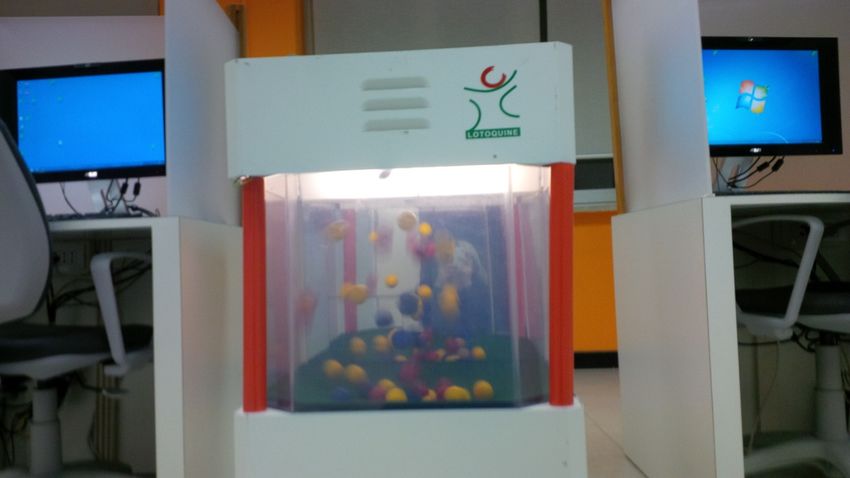
7 The Bingo Blower is a rectangular-shaped, glass-sided: inside the glass walls are a set of pink, yellow, and blue balls in
continuous motion being moved about by a jet of wind from a fan in the base (see the picture in Appendix A). In addition,
during the sessions’ images of the Bingo Blower in action are projected via videocamera onto two big screens in the
laboratory. Subjects are free at any stage to get closer to the Blower to examine it as much as they want. All the balls inside
the Blower can at all times be seen by people outside, but, unless the number of balls in the Blower is low, the number
of balls of differing colors cannot be counted because they are continually moving around: while objective probabilities
do exist, subjects cannot know them. In this way, as noted by Hey and Pace (2014) [58], there is a “situation of genuine
ambiguity which eliminates the problem of suspicion; the problem of using directly a second-order probability distribution;
and the problem of using real events, therefore keeping the problem more similar to the original Ellsberg one”.Games 2019, 10, 9 14 of 22
Third, subjects have to guess whether their score in task B is higher, equal or lower than the
average score in the session. They earn W6 tokens if they are correct. This guess identifies subjects’
ex-post placement in the low-competence task.
Fourth, subjects have to estimate the temperature in New York City on a specific past date and
time (17 September 2014, at noon) and choose between betting on the correctness of their answer (they
win if they over/underestimate by one degree Celsius at the maximum) or on a 50/50 lottery. In both
lotteries, they win W7 or get zero. This choice captures subjects’ preference for external ambiguity (based
on an exogenous source, i.e., a measure of overestimation) with respect to risk. Furthermore, subjects
have to guess whether their estimation of NYC temperature is more, equally or less correct than the
average temperature estimated in the session. This guess identifies subjects’ ex-ante estimation in case
of external ambiguity.
Fifth, subjects have to estimate the number of yellow balls in the Bingo Blower and choose between
betting on the correctness of their answer (they win if they over/underestimate by one ball at the
maximum) or on a 50/50 lottery. In both lotteries, they again win W7 or get zero. This choice captures
another form of subjects’ preference for external ambiguity based on an exogenous source, the Bingo
Blower, with respect to risk. This time, however, subjects could feel to have some kind of “control”
and/or direct experience with the source of external ambiguity since the Bingo Blower was located
in the room where the experimental sessions took place and subjects could observe it as long as they
wanted and get as close to it as they liked in order to increase their perceived accuracy in estimating
the number of yellow balls. This guess identifies subjects’ ex-ante estimation in case of external ambiguity.
Furthermore, subjects have to guess whether their estimation of the number of yellow balls is more,
equally or less correct than the average number estimated in the session.
Stage 4. Subjects receive feedback on their total amount of earnings and decide how many
tokens—of the sum earned in the previous stages and that we call endowment Di , different for each
subject i—they want to allocate between two pairs of lotteries (“Pair 1” and “Pair 2” respectively):
they will decide the allocation of the tokens they earned for both pairs, but only one pair will be
selected at random and actually played. The structure of this “investing gamble” is grounded on
Gneezy and Potters (1997) [59].
Pair 1:
• Investment Choice 1a: subjects have to decide how many tokens (Gi ) out of their endowment Di
that they want to allocate to a lottery where the probability of winning 2.5 Gi (instead of getting
zero) corresponds to the percentile corresponding to their performance in task B.
• Investment Choice 1b: subjects have to decide how many tokens (Hi ) out of their endowment Di
that they want to allocate to a lottery where they win 2.5 Hi (instead of getting zero) if a yellow
ball is drawn from the Bingo Blower.
Obviously, the condition Gi + Hi ≤ Di must hold.
The ratio Gi /Hi in Pair 1 captures subjects’ preference for investing in internal ambiguity (based on
placement) in the low-competence task instead of investing in external BB-ambiguity.
Pair 2:
• Investment Choice 2a: subjects have to decide how many tokens (Gi ) out of their endowment
Di that they want to allocate to a lottery where the probability of winning 2.5 Gi is 12 and the
probability of getting 0 is 12 .
• Investment Choice 2b: subjects have to decide how many tokens (Hi ) out of their endowment Di
that they want to allocate to a lottery where they win 2.5 Hi (instead of getting zero) if a yellow
ball is drawn from the Bingo Blower.
Again, the condition Gi + Hi ≤ Di must hold.
The ratio Gi /Hi in Pair 2 captures subjects’ preference for investing in external BB-ambiguity vs. risk.
Finally, subjects have to estimate the number of yellow balls in the bingo-blower. They win W8 if
they over/underestimate by one ball at the maximum. This is to capture how correct subjects are whenYou can also read