Melt in Antarctica derived from Soil Moisture and Ocean Salinity (SMOS) observations at L band
←
→
Page content transcription
If your browser does not render page correctly, please read the page content below
The Cryosphere, 14, 539–548, 2020
https://doi.org/10.5194/tc-14-539-2020
© Author(s) 2020. This work is distributed under
the Creative Commons Attribution 4.0 License.

Melt in Antarctica derived from Soil Moisture and Ocean Salinity
(SMOS) observations at L band
Marion Leduc-Leballeur1,2 , Ghislain Picard2 , Giovanni Macelloni1 , Arnaud Mialon3 , and Yann H. Kerr3
1 Institute
        of Applied Physics “Nello Carrara”, National Research Council, 50019 Sesto Fiorentino, Italy
2 UGA,CNRS, Institut des Géosciences de l’Environnement (IGE), UMR 5001, 38041 Grenoble, France
3 CESBIO, CNES–CNRS–IRD–UPS, University of Toulouse, 31401 Toulouse CEDEX 09, France

Correspondence: Marion Leduc-Leballeur (m.leduc@ifac.cnr.it)

Received: 20 August 2019 – Discussion started: 20 September 2019
Revised: 15 December 2019 – Accepted: 9 January 2020 – Published: 11 February 2020

Abstract. Melt occurrence in Antarctica is derived from L-        ture and surface energy budget (e.g. Liu et al., 2006; Picard
band observations from the Soil Moisture and Ocean Salin-         et al., 2007). Moreover, intense melting has been identified
ity (SMOS) satellite between the austral summer 2010–2011         as a precursor of some major ice shelf collapses (Scambos
and 2017–2018. The detection algorithm is adapted from            et al., 2000). Thus, monitoring of the melt season contributes
a threshold method previously developed for 19 GHz pas-           to characterizing the seasonal and interannual climatic vari-
sive microwave measurements from the special sensor mi-           ations in Antarctica and is important for assessing the future
crowave imager (SSM/I) and special sensor microwave im-           stability of the ice sheet (Golledge et al., 2015).
ager sounder (SSMIS). The comparison of daily melt oc-               Remote sensing offers a particularly relevant means to ob-
currence retrieved from 1.4 and 19 GHz observations shows         tain information over the entire Antarctic continent and over
an overall close agreement, but a lag of few days is usu-         long-term periods, given the very rare in situ measurements
ally observed by SMOS at the beginning of the melt season.        related to melt or liquid water (Jakobs et al., 2019). Mi-
To understand the difference, a theoretical analysis is per-      crowave frequencies have been widely used to detect melt
formed using a microwave emission radiative transfer model.       in polar regions, exploiting the marked variation in the sig-
It shows that the sensitivity of 1.4 GHz signal to liquid wa-     nal due to the high absorption of microwaves by water rel-
ter is significantly weaker than at 19 GHz if the water is only   ative to that of dry snow. Various detection algorithms have
present in the uppermost tens of centimetres of the snow-         been developed for active sensors (e.g. Nghiem et al., 2001,
pack. Conversely, 1.4 GHz measurements are sensitive to wa-       2005; Ashcraft and Long, 2006; Kunz and Long, 2006; Hall
ter when spread over at least 1 m and when present in depths      et al., 2009; Trusel et al., 2012; Zheng et al., 2019) and pas-
up to hundreds of metres. This is explained by the large          sive sensors (e.g. Mote et al., 1993; Ridley, 1993; Zwally
penetration depth in dry snow and by the long wavelength          and Fiegles, 1994; Abdalati and Steffen, 1997; Torinesi et al.,
(21 cm). We conclude that SMOS and higher-frequency ra-           2003; Liu et al., 2005, 2006; Tedesco, 2007; Tedesco et al.,
diometers provide interesting complementary information on        2007) and applied to the Greenland and Antarctic ice sheets.
melt occurrence and on the location of the water in the snow-        In the case of radiometer measurements, studies have
pack.                                                             mainly used 19 and 37 GHz frequencies available since 1979
                                                                  from several satellite sensors such as the scanning multichan-
                                                                  nel microwave radiometer (SMMR) on the Nimbus 7 satel-
                                                                  lite or the special sensor microwave imager (SSM/I) and spe-
1   Introduction                                                  cial sensor microwave imager sounder (SSMIS) from the De-
                                                                  fense Meteorological Satellite Program (DMSP) satellites.
Melt occurs in coastal Antarctica and on ice shelves during       Since 2009, the Soil Moisture and Ocean Salinity (SMOS)
the austral summer. Its duration and extent are useful cli-       satellite has provided radiometric observations at the L band,
mate indicators due to their connection to surface tempera-

Published by Copernicus Publications on behalf of the European Geosciences Union.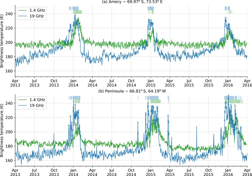
540                            M. Leduc-Leballeur et al.: Melt in Antarctica derived from SMOS observations at L band

a frequency capable of penetrating much deeper into the ice       at: https://nsidc.org/data/nsidc-0609, last access: 9 February
sheets, on the order of several hundred metres at 1.4 GHz         2020).
(Passalacqua et al., 2018) compared to only a few metres for
the higher frequencies (Surdyk, 2002). This suggests that L-      2.2    Observations at 19 GHz and daily surface melting
band observations could offer new information on melt.
   The aim of this study is to retrieve melt in Antarctica from   Satellite observations at 19 GHz were acquired by the SSM/I
daily SMOS observations and to investigate the similarities       and Special SSMIS, processed by the National Snow and Ice
and differences with melt detected at 19 GHz. Section 2 in-       Data Center (NSIDC; Maslanik and Stroeve, 2004).
troduces the datasets. Section 3 describes the method for            Daily TB observations at H polarization are processed ac-
detecting melt, and Sect. 4 compares the daily melt occur-        cording to Picard and Fily (2006) to derive daily surface
rence obtained with 1.4 and 19 GHz observations. Section 5        melt from 1979 to 2018 (available at: http://gp.snow-physics.
presents a modelling study to assess the liquid water sensitiv-   science/melting last access: 9 February 2020). This dataset
ity of brightness temperature (TB ) at 1.4 GHz and to discuss     provides daily melt status, i.e. presence or absence of liq-
the differences with 19 GHz.                                      uid water, for every grid point on the southern stereographic
                                                                  polar grid with a grid spacing of 25 km2 . The effective reso-
                                                                  lution of the product is coarser, of the order of 40 km, close
                                                                  to that provided by SMOS.
2     Datasets                                                       To compare SMOS and SSMIS datasets, the SSMIS ob-
                                                                  servations and products are collocated within the SMOS grid
2.1    SMOS observations                                          using the nearest neighbour method. If the nearest neighbour
                                                                  is not flagged as “land” in the SSMIS grid, the pixel was re-
The SMOS mission was developed by the European Space              moved from the analysis to avoid the error of comparison
Agency (ESA) in collaboration with the Centre National            between the two frequencies. In this way, about 50 pixels are
d’Études Spatiales (CNES) in France and the Centro para           excluded, which does not affect the statistical significance of
el Desarrollo Tecnológico Industrial (CDTI) in Spain. This        the comparison results.
satellite is operated by CNES and ESA and carries on board
a L-band interferometric radiometer operating at 1.4 GHz
(21 cm) with an averaged ground resolution of 43 km (Kerr         3     Melting detection method
et al., 2010). The radiometer provides multi-angular fully po-
larized TB (Kerr et al., 2001).                                   The algorithm for detecting melt occurrence from the
    The SMOS Level 3 product delivers multi-angular TB at         1.4 GHz observations is inspired by the work at 19 GHz of
the top of the atmosphere in the antenna polarization refer-      Torinesi et al. (2003), itself based on Zwally and Fiegles
ence frame (Al Bitar et al., 2017). The product is georef-        (1994). The algorithm determines an optimal threshold for
erenced on the Equal-Area Scalable Earth version 2.0 grid         every year in every pixel and considers that any daily TB H
(EASE-Grid 2; Brodzik et al., 2012), with an oversampled          over this threshold indicates melting occurrence. TB is mea-
resolution of about 628 km2 , which is distorted in the po-       sured at large observation angles (above 50◦ ). In this configu-
lar regions (around 100 km×6 km as latitude × longitude).         ration, the H polarization is favoured because the emissivity
It comprises the daily average and incident-angle average,        of dry firn is usually significantly lower at H than at V po-
with angle bins every 5◦ from 0 to 65◦ . TB values at vertical    larization, while the emissivity of wet firn is always close to
(V ) and horizontal (H ) polarizations for the 50–55◦ aver-       1 at both polarizations. It results in the increase in TB from
age range of incidence angle are used here. They come from        dry to wet snow being more significant at H polarization and
the RE04 reprocessed version between April 2010 and April         easier to detect.
2015 and from the operational version between May 2015               The algorithm uses an adaptive threshold T in each grid
to March 2018, both distributed by CATDS (Centre Aval de          point and for each year given by T = M + aσ , with M being
Traitement des Données SMOS; https://www.catds.fr/, last          the time average and σ the standard deviation of TB when
access: 9 February 2020).                                         snow is dry. According to the analysis of daily air surface
    The gaps shorter than 3 d in the SMOS time series are         temperature, Torinesi et al. (2003) found a suitable value of
filled by a linear interpolation. Longer gaps result in miss-     a = 3 so that most melting events correspond to daily max-
ing values in the product. If more than 60 d are missing over     imum temperatures above −5 ◦ C. This value is also typical
a year, the grid point is ignored for that year (about 7 % of     for outlier detection (e.g. von Storch and Zwiers, 2001).
pixel every year, mainly south of 83◦ S).                            To solve the circular problem of computing M and σ for
    The land–ocean mask used comes from the Land-Ocean-           non-melting days in order to detect melting days, the initial
Coastline-Ice classification associated with the EASE-            step consists of calculating M in each grid point on a fixed
Grid 2.0 map projections and derived from the MODIS land          period of 1 year – from 1 April to 31 March – and in setting
cover product by Brodzik and Knowles (2011) (available            aσ to a first-guess fixed value. Previous studies for 19 GHz

The Cryosphere, 14, 539–548, 2020                                                      www.the-cryosphere.net/14/539/2020/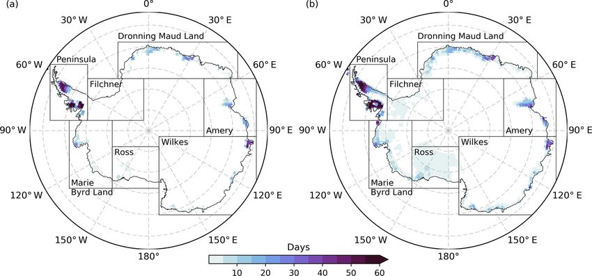
M. Leduc-Leballeur et al.: Melt in Antarctica derived from SMOS observations at L band 541
used aσ = 30 K. However, we found it unsuitable at 1.4 GHz January at 250 000 and 110 000 km2 for 19 and 1.4 GHz, re-
because of the weaker sensitivity to liquid water (Sect. 5). spectively. Spatial variations are illustrated by Fig. 3, which
We instead propose a lower first-guess value of aσ = 15 K. shows the annual mean duration of the melt season between
With these assumptions, a first-guess melt time series is April 2010 and March 2018 detected at both frequencies.
detected, and new estimates of M and σ are computed by Melting is concentrated on the coast, with a maximum in
removing melting days from the TB series, still limiting the the Antarctic Peninsula, as previously reported for 19 GHz
period from 1 April and 31 March. Melt is then detected once (Tedesco, 2009; Kuipers Munneke et al., 2012; Datta et al.,
again using the updated threshold. The process is iterated 2018, 2019; Scott et al., 2019). The largest differences are
three times to ensure stable estimates. The algorithm returns observed in the Filchner and Ross ice shelves, where melt is
a binary indicator for each day and each grid point, 0 for the detected to occur on a few days every year at 19 GHz but is
absence and 1 for the presence of liquid water. insufficient to be detected at 1.4 GHz. The difference is cer-
This algorithm needs further correction for some false tainly explained by the difference of sensitivity. Indeed, as
alarms found on the Antarctic Plateau, where melt is known these ice shelves only experience limited melt, the liquid wa-
to never occur. These alarms are likely due to variations in ter is likely concentrated in the uppermost few centimetres of
TB H of the order of several kelvin that were reported by the snowpack.
Brucker et al. (2014) and Leduc-Leballeur et al. (2017) and Figures 3 and 4 highlight that 19 GHz is more effective for
are explained to result from the snow metamorphism and sur- detecting short melting duration than 1.4 GHz. Indeed, more
face hoar removal by wind storms. Noting that these changes than 55 % of the pixels where melt occurs remain wet for less
do not impact TB V , although melt does, we consider here than 10 d in a year, according to 19 GHz observations, and
that the areas with low annual standard deviation of TB V are about 20 % remain wet between 11 and 20 d. At 1.4 GHz, the
not subject to melt. We estimated a threshold standard devi- duration of the melt season is usually longer. In only 20 % of
ation of 2.8 K based on the fact that it excludes 95 % of grid the pixels subject to melt, the season is 1–10 d; it is 11–40 d
points with surface elevation higher than 1500 m. Thus, as a in 55 % of the pixels. This hints at the fact that SMOS is only
final step of the algorithm, the grid points with a TB V annual sensitive to long and intense melt seasons.
standard deviation lower than this threshold are masked out However, it also happens that some melting days are de-
for that year. tected with the 1.4 GHz observations but not with the 19 GHz
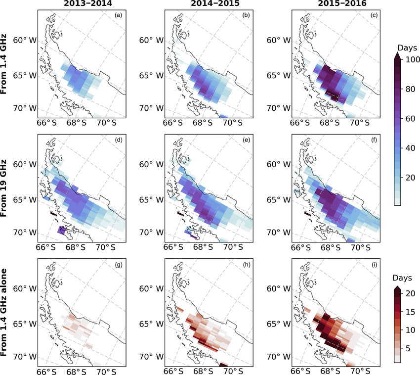
observations. This case is illustrated with the example of the
Antarctic Peninsula provided in Fig. 5 for the three sum-
4 Comparison with 19 GHz mer seasons from 2013 to 2016. This area is known to be
subjected each year to a long melt season, but high inter-
Figure 1 shows two examples of two consecutive melt sea- annual variability is observed. Zheng et al. (2019) studied
sons in the Amery area (69.97◦ S, 73.53◦ E) and the Antarctic the Antarctic Peninsula with a satellite radiometer and scat-
Peninsula (66.81◦ S, 64.19◦ W). For each event, melt is de- terometer as well as a climate model. They found that over
tected several days earlier at 19 GHz compared to 1.4 GHz. the period 2010–2017 the lowest wet-snow extent is observed
For instance, in 11 December 2013 in the Amery time series, during the 2013–2014 summer season, whereas the largest is
a short melting event lasting for 6 d is missed at 1.4 GHz, observed during 2015–2016. These two particular events are
while it is well detected at 19 GHz. This suggests that this also retrieved by SMOS and SSMIS during this period.
event was weak and only affected the superficial part of the Figure 5g, h and i show the number of days detected as
snowpack. On the other hand, the short melting event dur- melting at 1.4 GHz but being dry at 19 GHz. In 2013–2014,
ing March 2015 in the peninsula time series is detected by 2.6 d on average are only detected as melting by SMOS over
both frequencies, suggesting intense melt with percolation in a surface of 35 625 km2 (57 pixels). In 2015–2016, 12.3 d on
a large upper part of the snowpack. average are only detected as melting by SMOS over a surface
The beginning of the melt season detected usually largely of 83 125 km2 (133 pixels), which is 57 % and 24 % larger
differs between both frequencies, as illustrated in Fig. 2. On than in 2013–2014 and 2014–2015, respectively. As 2015–
average, the first melting day can be detected as early as 2016 is known to have been subjected to an intensive melt-
September at 19 GHz, while it is rare to detect melt earlier ing event in the Antarctic Peninsula due to a strong El Niño
than December at 1.4 GHz. For the pixel where melt is de- event (Nicolas et al., 2017), this could suggest that 1.4 GHz
tected by both frequencies in a given year, the 19 GHz de- provides additional information to 19 GHz in the case of in-
tection precedes the 1.4 GHz detection by 1–5 d for 28 % of tense melting events. In this way, Wiesenekker et al. (2018)
the pixels and by 6–15 d for 26 % of them. This lag is also showed that a stronger-than-normal foehn wind, which is a
observed for the end of the season, with a persistence of the hot, dry wind on the downwind side of a mountain range,
melt detected at 1.4 GHz until nearly April. happens over the peninsula in 2015–2016. This generates
Figure 2 also highlights that the melt extent detected at an increase in melt near the foot of the Antarctic Peninsula
19 GHz is 3 to 6 times as large as at 1.4 GHz, depending mountains. This area matches the pixels where 1.4 GHz ob-
on the years. The standard deviation maximum is reached in servations detected more than 20 d not detected by 19 GHz
www.the-cryosphere.net/14/539/2020/ The Cryosphere, 14, 539–548, 2020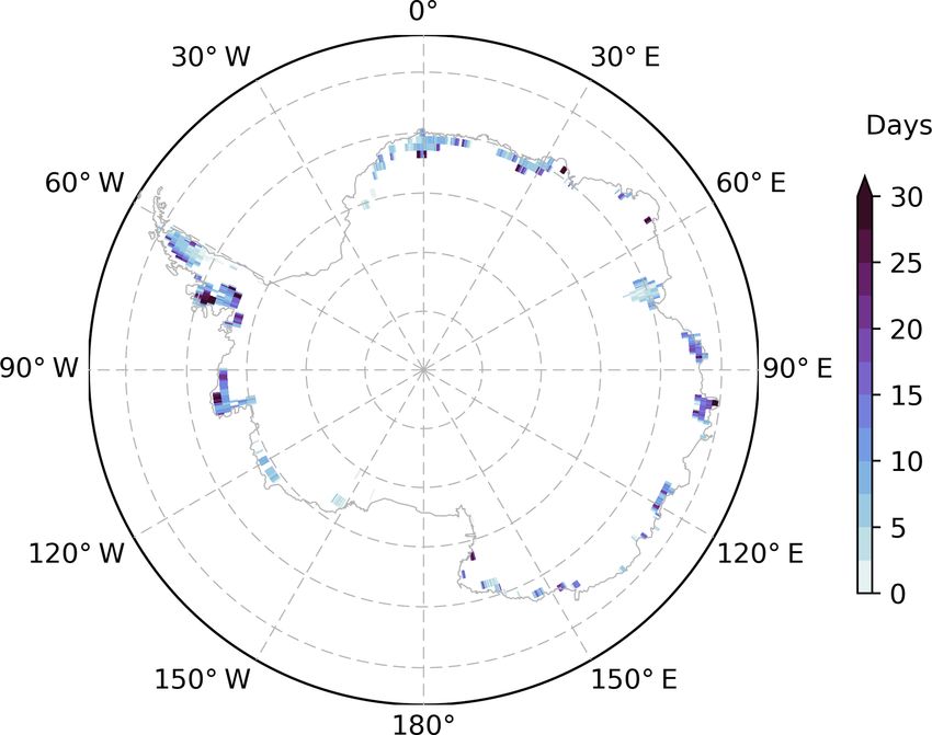
542                             M. Leduc-Leballeur et al.: Melt in Antarctica derived from SMOS observations at L band

Figure 1. Brightness temperature at H polarization (K) at 1.4 GHz (green) and 19 GHz (blue) from April 2013 to March 2016 at (a) the
Amery area and (b) the Antarctic Peninsula. The melting days detected by each frequency are depicted by crosses on the time series and
recalled by pale lines above.

                                                                     information about a part of snowpack in depth which is not
                                                                     reached by SSMIS observations.
                                                                        Figure 6 maps, for the whole continent, the mean number
                                                                     of melting days detected at 1.4 GHz without concurrent de-
                                                                     tection at 19 GHz during summer season over our dataset. It
                                                                     shows that the geographical distribution is related to the total
                                                                     number of melt events (Fig. 3), meaning that all the areas are
                                                                     concerned by the differential detection at both frequencies.
                                                                     On average, 10 ± 8 d are detected only by SMOS. Moreover,
                                                                     over a total of about 117 000 melting days, taking all pixels
                                                                     and summer seasons together that were detected at 1.4 GHz,
                                                                     28 % are not concurrently detected at 19 GHz. These melting
                                                                     days happen on 1 February ±23 d on average, i.e. at the end
Figure 2. Daily mean melting extent from April 2010 to March
2018 detected with observations at 1.4 GHz (green) and at 19 GHz
                                                                     of summer season. Conversely, over 225 000 melting days
(blue). Standard deviation is in pale area.                          are detected by 19 GHz during the same period, and 66 % are
                                                                     not concurrently detected at 1.4 GHz.

                                                                     5   Sensitivity to liquid water content
(Fig. 5). Moreover, Datta et al. (2019) also found that high
melt occurrence induced by foehn wind is observed in 2015–           The sensitivity to liquid water at 1.4 GHz is investigated in
2016, and they highlighted that this foehn wind increases the        order to understand the signal variations observed in Antarc-
meltwater percolation by up 2 m in depth along the moun-             tica and to investigate the observed differences with the
tains. This suggests that SMOS observations could provide            19 GHz melt detection.

The Cryosphere, 14, 539–548, 2020                                                          www.the-cryosphere.net/14/539/2020/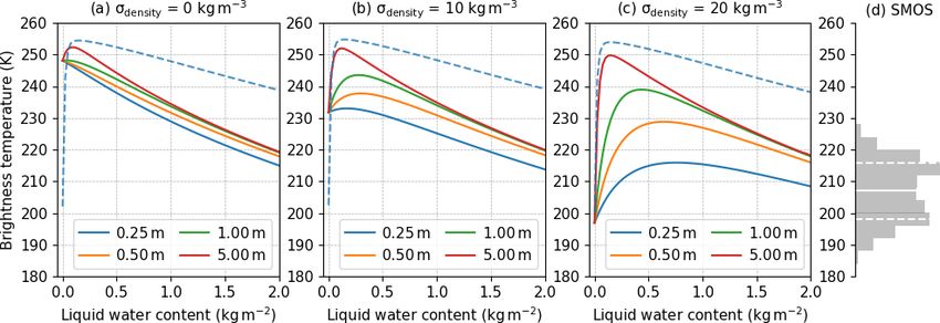
M. Leduc-Leballeur et al.: Melt in Antarctica derived from SMOS observations at L band                                         543

Figure 3. Annual mean of melting duration (days) from April 2010 to March 2018 detected with observations (a) at 1.4 GHz (SMOS) and
(b) at 19 GHz (SSMIS). Seven regions are outlined.

                                                                    is 273 K from the surface to 5 m in depth, then constant at
                                                                    263 K up to 500 m depth and, finally, linearly increases to
                                                                    reach 273 K at the bottom. Density linearly increases from
                                                                    300 kg m−3 at the surface to 917 kg m−3 at 100 m in depth
                                                                    and is constant below (Leduc-Leballeur et al., 2015). Grain
                                                                    size is constant, at 1 mm. Picard et al. (2013) showed that
                                                                    grain size has an effect on the sensitivity to LWC at 19 GHz.
                                                                    Nevertheless, it is not expected at 1.4 GHz because the wave-
                                                                    length is much larger than grain size and scattering by grains
                                                                    can be neglected (Mätzler, 1987).

                                                                    5.2   Effect of snow density vertical variability

Figure 4. Annual melting duration distribution of wet pixels de-    By modelling L-band emission at Dome C on the Antarctic
tected with 1.4 GHz (solid green) and 19 GHz (hatched blue) over    Plateau, Leduc-Leballeur et al. (2015) highlighted that layer-
the whole continent of Antarctica for each summer season from       ing must be considered to obtain reliable TB estimation. To
2010 to 2018.                                                       assess if this is also the case for wet snow, the simulations
                                                                    are performed with a smooth density profile and two density
                                                                    profiles with an added Gaussian noise of a standard devia-
5.1   Microwave emission modelling                                  tion of 10 and 20 kg m−3 , respectively, between the surface
                                                                    and 300 m in depth. Figure 7 shows the DMRT-ML simula-
TB is simulated with the multi-layered dense-medium radia-          tions at both 1.4 and 19 GHz as a function of LWC and for
tive theory model (DMRT-ML; Picard et al., 2013), avail-            various thicknesses of wet snow.
able at: http://gp.snow-physics.science/dmrtml (last access:           For the dry snowpack (LWC = 0 kg m−2 ), the layering sig-
9 February 2020). This model is based on the radiative trans-       nificantly decreases TB H from 248.1 K for the smooth den-
fer theory (Tsang and Kong, 2001). The snowpack is rep-             sity profile to 231.8 and 196.9 K for the density profiles with
resented by a stack of snow horizontal layers defined by            a standard deviation of 10 and 20 kg m−3 , respectively. In
their thickness, temperature, density, grain size and liquid        the wet-snow condition, the layering effect becomes weaker
water content (LWC). Simulations are performed at 1.4 and           as the LWC increases and is insignificant (< 4 K variations)
19 GHz, with an incidence angle of 55◦ .                            for LWC larger than 1 kg m−2 or when water is spread over
   Synthetic snowpack is assumed to run simulations. It has         a large thickness. Thus, between dry and wet conditions, the
a total thickness of 1000 m and is divided into layers of 5 cm      TB H difference increases with the layering.
from the surface to 500 and 50 m below. The temperature

www.the-cryosphere.net/14/539/2020/                                                         The Cryosphere, 14, 539–548, 2020
544 M. Leduc-Leballeur et al.: Melt in Antarctica derived from SMOS observations at L band
Figure 5. Annual melting duration (days) over the Antarctic Peninsula detected with observations (a–c) at 1.4 GHz and (d–f) at 19 GHz from
2013–2014 to 2015–2016. (g–i) Number of days detected as melting at 1.4 GHz but dry at 19 GHz.
ness is 1000 ± 50 m to match with the snowpack config-
uration used for simulations. The SMOS TB H average is
206.9 ± 8.9 K. This suggests that simulations with a density
variability lower than 10 kg m−3 overestimate the dry TB H
and thus underestimate the variations between dry and wet
snow at 1.4 GHz. We thus now consider the case of a density
variability of 20 kg m−3 only.
The simulations show that TB H at 1.4 GHz increases from
dry to wet by 19 K when the wet-snow layer is 0.25 m and
53 K when it is 5 m (Fig. 7c). While in both cases, the change
is high and detectable, this highlights not only the impor-
tance of the total column amount of liquid water but also that
of the distribution at depth. Additionally, Fig. 7c shows that
the maximum increase in TB H is reached for LWC of 0.75
and 0.15 kg m−2 , respectively, for the 0.25 and 5 m thick wet-
snow layers. This means that the LWC sensitivity of 1.4 GHz
Figure 6. Mean melting days by summer season detected as melting TB H is weaker when liquid water is confined to the upper-
at 1.4 GHz but dry at 19 GHz. most tens of centimetres of the snowpack. This is the ratio-
nale for choosing a lower first-guess aσ for the detection al-
gorithm at 1.4 GHz than at the higher frequencies (Sect. 3).
Figure 7d shows daily SMOS TB H from June to August Additionally, Fig. 7c shows that regardless of the wet-layer
– a period when snow is expected to always be dry – in thickness, TB H reaches a maximum at a certain LWC value,
2010–2018. The histogram only includes pixels where melt- which decreases when the wet layer becomes thicker. Thus,
ing has been detected at least once and where ice thick-
The Cryosphere, 14, 539–548, 2020 www.the-cryosphere.net/14/539/2020/M. Leduc-Leballeur et al.: Melt in Antarctica derived from SMOS observations at L band 545
Figure 7. (a–c) DMRT-ML brightness temperature at H polarization (K) as a function of liquid water content for several wet-snow thick-
nesses in the upper snowpack (colours) at 1.4 GHz (solid lines) and 0.25 m of wet snow at 19 GHz (dashed line), with three density variabil-
ities (σdensity ). (d) Daily winter SMOS observations distribution (see text for details), with mean (white solid) and standard deviation (white
dashed).
an increase in LWC is not detectable because of the TB sat-
uration. This jeopardizes the possibility of using microwave
observations to estimate LWC values or even the wet-layer
thickness.
By contrast, at 19 GHz, the density variability has no ef-
fect, and the TB H variations are mainly driven by LWC.
A sharp increase of 54 K is observed, and the maximum is
reached for LWC of 0.15 kg m−2 . The thickness of the wet-
snow layer has no effect (not shown in Fig. 7c).
In conclusion, these simulations show that 19 GHz is more
sensitive to liquid water than at 1.4 GHz and that other factors
such as the vertical distribution of the water or the layering
have a smaller influence. This indicates that detection of melt Figure 8. DMRT-ML brightness temperature at H polarization (K)
occurrence at the surface is more robust at 19 GHz. for 55◦ of incidence angle as a function of the wet-snow-layer depth
within the snowpack for a wet-layer thickness of 1 m at 1.4 GHz
5.3 Effect of the wet-snow depth (green) and 0.1 m at 19 GHz (blue). Values for a dry snowpack are
in dashed lines.
We explore here the situation when the wet-snow layer is
buried under a layer of dry firn. This corresponds to the end
of summer, when the snowpack freezes up from the surface, at this frequency if the water percolates deep into the firn.
or on the ice shelves, where meltwater enters the crevasses However, observations at 19 GHz should still be suitable for
and accumulates at depth. The simulations are performed the detection of remnant liquid water at the end of the season
with a wet-snow layer (0.2 kg m−2 ), progressively moving and when the snowpack is continuous, i.e. without crevasse.
down from the surface to 400 m in depth. The wet-layer These results suggest that despite a lower sensitivity at
thickness is 1 m at 1.4 GHz and 0.1 m at 19 GHz to moderate 1.4 GHz, liquid water could be detected with SMOS up to
the sensitivity effect presented in the previous section. Re- several tens of metres at depth, and this is new information
sults highlight that TB H is maximum when wet snow is at the compared to that provided by the existing melt product de-
surface for both frequencies and decreases within a few me- rived from 19 GHz and higher-frequency observations. The
tres at 19 GHz and more gradually at 1.4 GHz (Fig. 8). TB H difference observed between 19 and 1.4 GHz could be ex-
is still more than 10 K higher than in dry conditions when the ploited to determine if the melt event was limited to the few
wet layer is at 60 m in depth at 1.4 GHz. Deeper than 100 m, first centimetres of snowpack or if water percolated over a
the difference between dry and wet TB H is lower than 3 K, sufficient thickness to be detected by SMOS.
i.e. lower than the noise level with SMOS.
At 19 GHz, the simulation shows a TB H variation of 2 K
between dry and wet when the wet snow is at 5 m in depth.
Thus, the sensitivity to liquid water is relatively quickly lost
www.the-cryosphere.net/14/539/2020/ The Cryosphere, 14, 539–548, 2020546 M. Leduc-Leballeur et al.: Melt in Antarctica derived from SMOS observations at L band
6 Conclusions Financial support. This research has been supported by the ESA
support through the CryoSMOS project (contract 4000112262/14/I-
The L-band brightness temperature (TB ) from the SMOS NB) and the French space agency (CNES) support through the
satellite has been explored to retrieve information about the SMOS TOSCA project.
melt season in Antarctica. Daily melt occurrence can be re-
trieved using previously developed algorithms for higher fre-
quencies (Zwally and Fiegles, 1994; Torinesi et al., 2003) af- Review statement. This paper was edited by Chris Derksen and re-
ter a slight adaptation to account for the lower sensitivity at viewed by two anonymous referees.
1.4 GHz. The comparison of melt detected at 1.4 and 19 GHz
(Picard and Fily, 2006) shows a lower rate of detection at
1.4 GHz. In particular, SMOS misses short, probably weak, References
events, which are in contrast perfectly detected by SSMIS.
A theoretical analysis has been performed using a snow- Abdalati, W. and Steffen, K.: Snowmelt on the Greenland
pack emission radiative transfer model (DMRT-ML) in order ice sheet as derived from passive microwave satellite data,
to estimate the sensitivity of TB at 1.4 and 19 GHz to liq- J. Climate, 10, 165–175, https://doi.org/10.1175/1520-
uid water content (LWC) and water distribution in the snow- 0442(1997)0102.0.CO;2, 1997.
pack. As expected from previous studies, a clear increase in Al Bitar, A., Mialon, A., Kerr, Y. H., Cabot, F., Richaume, P.,
Jacquette, E., Quesney, A., Mahmoodi, A., Tarot, S., Parrens,
TB happens when snow becomes wet. However, the simula-
M., Al-Yaari, A., Pellarin, T., Rodriguez-Fernandez, N., and
tions clearly demonstrate that 1.4 GHz is less sensitive than
Wigneron, J.-P.: The global SMOS Level 3 daily soil moisture
19 GHz, especially when liquid water stays within the top and brightness temperature maps, Earth Syst. Sci. Data, 9, 293–
centimetres of the snowpack. A thick wet layer (> about 315, https://doi.org/10.5194/essd-9-293-2017, 2017.
0.5 m) is required to trigger a sharp and detectable TB in- Ashcraft, I. S. and Long, D. G.: Comparison of methods for
crease. Despite this limited sensitivity, the simulations show melt detection over Greenland using active and passive mi-
that 1.4 GHz is suitable to detect wet snow buried under a dry crowave measurements, Int. J. Remote Sens., 27, 2469–2488,
surface. For instance, an increase in TB higher than 10 K with https://doi.org/10.1080/01431160500534465, 2006.
respect to a dry snowpack can be observed with liquid water Brodzik, M. J. and Knowles, K.: EASE-Grid 2.0 Land-
at up to 60 m in depth, according to the simulation configu- Ocean-Coastline-Ice Masks Derived from Boston Uni-
ration. versity MODIS/Terra Land Cover Data, Version 1,
NASA National Snow and Ice Data Center Dis-
An avenue is a combined use of both frequencies to deter-
tributed Active Archive Center, Boulder, Colorado, USA,
mine if a melt event was limited to the surface of the snow-
https://doi.org/10.5067/VY2JQZL9J8AQ, 2011.
pack or if it was intense enough to inject water at depths. Brodzik, M. J., Billingsley, B., Haran, T., Raup, B., and Savoie,
However, further algorithmic work is needed to exploit this M. H.: EASE-grid 2.0: Incremental but Significant Improve-
possibility of deep-water detection with SMOS. ments for Earth-Gridded Data Sets, ISPRS Int. Geo-Inf., 1, 32–
45, https://doi.org/10.3390/ijgi1010032, 2012.
Brucker, L., Dinnat, E. P., Picard, G., and Champollion, N.: Effect of
Data availability. Data for daily occurrence of melt retrieved snow surface metamorphism on Aquarius L-band radiometer ob-
from SMOS are available at: https://www.catds.fr/Products/ servations at Dome C, Antarctica, IEEE T. Geosci. Remote, 52,
Available-products-from-CEC-SM/CryoSMOS-project (Picard 7408–7417, https://doi.org/10.1109/TGRS.2014.2312102, 2014.
and Leduc-Leballeur, 2020). Datta, R. T., Tedesco, M., Agosta, C., Fettweis, X., Kuipers
Munneke, P., and van den Broeke, M. R.: Melting over the
northeast Antarctic Peninsula (1999–2009): evaluation of a high-
Author contributions. MLL, GP and GM led the study and per- resolution regional climate model, The Cryosphere, 12, 2901–
formed the analysis. AM and YHK supported for using the SMOS 2922, https://doi.org/10.5194/tc-12-2901-2018, 2018.
observations. All authors contributed to the paper. Datta, R. T., Tedesco, M., Fettweis, X., Agosta, C., Lher-
mitte, S., Lenaerts, J., and Wever, N.: The Effect of Foehn-
Induced Surface Melt on Firn Evolution Over the North-
Competing interests. The authors declare that they have no conflict east Antarctic Peninsula, Geophys. Res. Lett., 46, 3822–3831,
of interest. https://doi.org/10.1029/2018GL080845, 2019.
Golledge, N. R., Kowalewski, D. E., Naish, T. R., Levy, R. H.,
Fogwill, C. J., and Gasson, E. G.: The multi-millennial Antarc-
tic commitment to future sea-level rise, Nature, 526, 421–425,
Acknowledgements. The SMOS L3 product comes from the
https://doi.org/10.1038/nature15706, 2015.
CATDS, managed for the CNES by IFREMER (Brest, France). We
Hall, D. K., Nghiem, S. V., Schaaf, C. B., DiGirolamo, N. E.,
would also like to thank the editor and the two anonymous review-
and Neumann, G.: Evaluation of surface and near-surface
ers for their very helpful comments.
melt characteristics on the Greenland ice sheet using MODIS
and QuikSCAT data, J. Geophys. Res.-Earth, 114 F04006,
https://doi.org/10.1029/2009JF001287, 2009.
The Cryosphere, 14, 539–548, 2020 www.the-cryosphere.net/14/539/2020/M. Leduc-Leballeur et al.: Melt in Antarctica derived from SMOS observations at L band 547 Jakobs, C. L., Reijmer, C. H., Kuipers Munneke, P., König-Langlo, Nghiem, S. V., Steffen, K., Neumann, G., and Huff, R.: Mapping of G., and van den Broeke, M. R.: Quantifying the snowmelt– ice layer extent and snow accumulation in the percolation zone albedo feedback at Neumayer Station, East Antarctica, The of the Greenland ice sheet, J. Geophys. Res.-Earth, 110, F02017, Cryosphere, 13, 1473–1485, https://doi.org/10.5194/tc-13-1473- https://doi.org/10.1029/2004JF000234, 2005. 2019, 2019. Nicolas, J. P., Vogelmann, A. M., Scott, R. C., Wilson, A. B., Kerr, Y. H., Waldteufel, P., Wigneron, J.-P., Martinuzzi, J., Font, Cadeddu, M. P., Bromwich, D. H., Verlinde, J., Lubin, D., Rus- J., and Berger, M.: Soil moisture retrieval from space: The Soil sell, L. M., Jenkinson, C., Powers H. H., Ryczek M., Stone G., Moisture and Ocean Salinity (SMOS) mission, IEEE T. Geosci. and Wille J. D.: January 2016 extensive summer melt in West Remote, 39, 1729–1735, https://doi.org/10.1109/36.942551, Antarctica favoured by strong El Niño, Nat. Commun., 8, 15799, 2001. https://doi.org/10.1038/ncomms15799, 2017. Kerr, Y. H., Waldteufel, P., Wigneron, J.-P., Delwart, S., Cabot, F., Passalacqua, O., Picard, G., Ritz, C., Leduc-Leballeur, M., Boutin, J., Escorihuela, M.-J., Font, J., Reul, N., Gruhier, C., Ju- Quiquet, A., Larue, F., and Macelloni, G.: Retrieval of glea, S. E., Drinkwater, M. R., Hahne, A., Martín-Neira, M., and the Absorption Coefficient of L-Band Radiation in Antarc- Mecklenburg, S.: The SMOS mission: New tool for monitoring tica From SMOS Observations, Remote Sensing, 10, 1954, key elements ofthe global water cycle, Proc. IEEE, 98, 666–687, https://doi.org/10.3390/rs10121954, 2018. https://doi.org/10.1109/JPROC.2010.2043032, 2010. Picard, G. and Fily, M.: Surface melting observations in Antarctica Kuipers Munneke, P., Picard, G., van den Broeke, M. R., Lenaerts, by microwave radiometers: Correcting 26-year time series from J. T. M., and van Meijgaard, E.: Insignificant change in Antarctic changes in acquisition hours, Remote Sens. Environ., 104, 325– snowmelt volume since 1979, Geophys. Res. Lett., 39, L01501, 336, https://doi.org/10.1016/j.rse.2006.05.010, 2006. https://doi.org/10.1029/2011GL050207, 2012. Picard, G. and Leduc-Leballeur, M.: Melting occurrence from Kunz, L. B. and Long, D. G.: Melt Detection in Antarc- SMOS observations, available at: https://www.catds.fr/Products/ tic Ice Shelves Using Scatterometers and Microwave Available-products-from-CEC-SM/CryoSMOS-project, last ac- Radiometers, IEEE T. Geosci. Remote, 44, 2461–2469, cess: 9 February 2020. https://doi.org/10.1109/TGRS.2006.874138, 2006. Picard, G., Fily, M., and Gallée, H.: Surface melting derived from Leduc-Leballeur, M., Picard, G., Mialon, A., Arnaud, L., Lefeb- microwave radiometers: a climatic indicator in Antarctica, Ann. vre, E., Possenti, P., and Kerr, Y.: Modeling L-band bright- Glaciol., 46, 29–34, 2007. ness temperature at Dome C in Antarctica and comparison with Picard, G., Brucker, L., Roy, A., Dupont, F., Fily, M., Royer, A., SMOS observations, IEEE T. Geosci. Remote, 53, 4022–4032, and Harlow, C.: Simulation of the microwave emission of multi- https://doi.org/10.1109/TGRS.2015.2388790, 2015. layered snowpacks using the Dense Media Radiative transfer the- Leduc-Leballeur, M., Picard, G., Macelloni, G., Arnaud, L., ory: the DMRT-ML model, Geosci. Model Dev., 6, 1061–1078, Brogioni, M., Mialon, A., and Kerr, Y.: Influence of https://doi.org/10.5194/gmd-6-1061-2013, 2013. snow surface properties on L-band brightness temperature at Ridley, J.: Surface melting on Antarctic Peninsula ice shelves de- Dome C, Antarctica, Remote Sens. Environ., 199, 427–436, tected by passive microwave sensors, Geophys. Res. Lett., 20, https://doi.org/10.1016/j.rse.2017.07.035, 2017. 2639–2642, https://doi.org/10.1029/93GL02611, 1993. Liu, H., Wang, L., and Jezek, K. C.: Wavelet-transform based edge Scambos, T. A., Hulbe, C., Fahnestock, M., and Bohlander, detection approach to derivation of snowmelt onset, end and du- J.: The link between climate warming and break-up of ice ration from satellite passive microwave measurements, Int. J. Re- shelves in the Antarctic Peninsula, J. Glaciol., 46, 516–530, mote Sens., 26, 4639–4660, 2005. https://doi.org/10.3189/172756500781833043, 2000. Liu, H., Wang, L., and Jezek, K. C.: Spatiotemporal variations of Scott, R. C., Nicolas, J. P., Bromwich, D. H., Norris, J. R., and snowmelt in Antarctica derived from satellite scanning multi- Lubin, D.: Meteorological drivers and large-scale climate forc- channel microwave radiometer and Special Sensor Microwave ing of West Antarctic surface melt, J. Climate, 32, 665–684, Imager data (1978–2004), J. Geophys. Res.-Earth, 111, F01003, https://doi.org/10.1175/JCLI-D-18-0233.1, 2019. https://doi.org/10.1029/2005JF000318, 2006. Surdyk, S.: Using microwave brightness temperature to detect Maslanik, J. and Stroeve, J.: DMSP SSM/I-SSMIS Daily short-term surface air temperature changes in Antarctica: An Polar Gridded Brightness Temperatures, Version 4, analytical approach, Remote Sens. Environ., 80, 256–271, NASA National Snow and Ice Data Center Dis- https://doi.org/10.1016/S0034-4257(01)00308-X, 2002. tributed Active Archive Center, Boulder, Colorado, USA, Tedesco, M.: Snowmelt detection over the Greenland ice sheet from https://doi.org/10.5067/AN9AI8EO7PX0, 2004, updated 2018. SSM/I brightness temperature daily variations, Geophys. Res. Mätzler, C.: Applications of the interaction of microwaves with Lett., 34, L02504, https://doi.org/10.1029/2006GL028466, 2007. the natural snow cover, Remote Sens. Rev., 2, 259–387, Tedesco, M.: Assessment and development of snowmelt retrieval https://doi.org/10.1080/02757258709532086, 1987. algorithms over Antarctica from K-band spaceborne brightness Mote, T. L., Anderson, M. R., Kuivinen, K. C., and Rowe, C. M.: temperature (1979–2008), Remote Sens. Environ., 113, 979– Passive microwave-derived spatial and temporal variations of 997, https://doi.org/10.1016/j.rse.2009.01.009, 2009. summer melt on the Greenland ice sheet, Ann. Glaciol., 17, 233– Tedesco, M., Abdalati, W., and Zwally, H.: Persistent sur- 238, https://doi.org/10.3189/S0260305500012891, 1993. face snowmelt over Antarctica (1987–2006) from 19.35 GHz Nghiem, S., Steffen, K., Kwok, R., and Tsai, W. Y.: Detec- brightness temperatures, Geophys. Res. Lett., 34, L18504, tion of snowmelt regions on the Greenland ice sheet us- https://doi.org/10.1029/2007GL031199, 2007. ing diurnal backscatter change, J. Glaciol., 47, 539–547, https://doi.org/10.3189/172756501781831738, 2001. www.the-cryosphere.net/14/539/2020/ The Cryosphere, 14, 539–548, 2020
548                               M. Leduc-Leballeur et al.: Melt in Antarctica derived from SMOS observations at L band

Torinesi, O., Fily, M., and Genthon, C.: Variability and trends of the   Zheng, L., Zhou, C., and Liang, Q.: Variations in Antarc-
  summer melt period of Antarctic ice margins since 1980 from              tic Peninsula snow liquid water during 1999–2017 re-
  microwave sensors, J. Climate, 16, 1047–1060, 2003.                      vealed by merging radiometer, scatterometer and model
Trusel, L. D., Frey, K. E., and Das, S. B.: Antarctic sur-                 estimations, Remote Sens. Environ., 232, 111219,
  face melting dynamics: Enhanced perspectives from radar                  https://doi.org/10.1016/j.rse.2019.111219, 2019.
  scatterometer data, J. Geophys. Res.-Earth, 117, F02023,               Zwally, J. H. and Fiegles, S.: Extent and duration of
  https://doi.org/10.1029/2011JF002126, 2012.                              Antarctic surface melting, J. Glaciol., 40, 463–475,
Tsang, L. and Kong, J. A.: Scattering of Electromagnetic Waves,            https://doi.org/10.3189/S0022143000012338, 1994.
  vol. 3: Advanced Topics, Wiley Interscience, New York, USA,
  2001.
von Storch, H. and Zwiers, F. W.: Statistical analysis in climate re-
  search, Cambridge University Press, Cambridge, UK, 2001.
Wiesenekker, J., Kuipers Munneke, P., Van den Broeke, M., and
  Smeets, C.: A Multidecadal Analysis of Föhn Winds over Larsen
  C Ice Shelf from a Combination of Observations and Model-
  ing, Atmosphere, 9, 172, https://doi.org/10.3390/atmos9050172,
  2018.

The Cryosphere, 14, 539–548, 2020                                                           www.the-cryosphere.net/14/539/2020/
You can also read